Bank Churn Exploration and Binary Classification

Contents

1. Introduction
2. Data Cleaning
3. Data Exploration
4. Feature Engineering
5. Modelling
6. Conclusion

---

1. Introduction

In this notebook we will explore a synthetic bank customer churn dataset used in a Kaggle community prediction competition, treating this like a real world problem and avoiding the use of any performance-boosting tricks that is are only specific to this competition dataset (i.e. utilizing data leakages due to the syntheticity of the data)

Churn - What and why?

Customer churn is a measure of how many customers leave the bank entirely. Customers may leave the bank due to many different reasons, a few common ones are: <ol> <li>Dissatisfaction with the products offered.</li> <li>Competitor offerings are more appealing.</li> <li>External factors that make it impossible for the customer to continue using the bank services.</li> </ol>

2. Data Cleaning

# Import packages and set styles
import pandas as pd
import numpy as np
import matplotlib.pyplot as plt
import seaborn as sns

from sklearn.preprocessing import MinMaxScaler, LabelEncoder
from sklearn.model_selection import train_test_split, GridSearchCV, KFold, cross_val_score
from sklearn.linear_model import LogisticRegression
from sklearn.ensemble import RandomForestClassifier
from xgboost import XGBClassifier
from lightgbm import LGBMClassifier
from sklearn.ensemble import VotingClassifier

from sklearn.pipeline import Pipeline
from sklearn.base import BaseEstimator, TransformerMixin
from sklearn.cluster import KMeans
from sklearn.metrics import classification_report, confusion_matrix, accuracy_score, f1_score, auc, roc_curve, roc_auc_score, make_scorer
import warnings
warnings.filterwarnings('ignore')

plt.style.use('fivethirtyeight')
sns.set_palette("muted")

df = pd.read_csv('train.csv')
df.head()

	id	CustomerId	Surname	CreditScore	Geography	Gender	Age	Tenure	Balance	NumOfProducts	HasCrCard	IsActiveMember	EstimatedSalary	Exited
0	0	15674932	Okwudilichukwu	668	France	Male	33.0	3	0.00	2	1.0	0.0	181449.97	0
1	1	15749177	Okwudiliolisa	627	France	Male	33.0	1	0.00	2	1.0	1.0	49503.50	0
2	2	15694510	Hsueh	678	France	Male	40.0	10	0.00	2	1.0	0.0	184866.69	0
3	3	15741417	Kao	581	France	Male	34.0	2	148882.54	1	1.0	1.0	84560.88	0
4	4	15766172	Chiemenam	716	Spain	Male	33.0	5	0.00	2	1.0	1.0	15068.83	0

df.shape

(165034, 14)

df.info()

<class 'pandas.core.frame.DataFrame'>
RangeIndex: 165034 entries, 0 to 165033
Data columns (total 14 columns):
 #   Column           Non-Null Count   Dtype  
---  ------           --------------   -----  
 0   id               165034 non-null  int64  
 1   CustomerId       165034 non-null  int64  
 2   Surname          165034 non-null  object 
 3   CreditScore      165034 non-null  int64  
 4   Geography        165034 non-null  object 
 5   Gender           165034 non-null  object 
 6   Age              165034 non-null  float64
 7   Tenure           165034 non-null  int64  
 8   Balance          165034 non-null  float64
 9   NumOfProducts    165034 non-null  int64  
 10  HasCrCard        165034 non-null  float64
 11  IsActiveMember   165034 non-null  float64
 12  EstimatedSalary  165034 non-null  float64
 13  Exited           165034 non-null  int64  
dtypes: float64(5), int64(6), object(3)
memory usage: 17.6+ MB

Column descriptions for the features within the dataset

1. Customer ID: A unique identifier for each customer
2. Surname: The customer’s surname or last name
3. Credit Score: A numerical value representing the customer’s credit score
4. Geography: The country where the customer resides (France, Spain or Germany)
5. Gender: The customer’s gender (Male or Female)
6. Age: The customer’s age.
7. Tenure: The number of years the customer has been with the bank
8. Balance: The customer’s account balance
9. NumOfProducts: The number of bank products the customer uses (e.g., savings account, credit card)
10. HasCrCard: Whether the customer has a credit card (1 = yes, 0 = no)
11. IsActiveMember: Whether the customer is an active member (1 = yes, 0 = no)
12. EstimatedSalary: The estimated salary of the customer
13. Exited: Whether the customer has churned (1 = yes, 0 = no)

print(df.duplicated().sum())
print(df.isna().sum())

0
id                 0
CustomerId         0
Surname            0
CreditScore        0
Geography          0
Gender             0
Age                0
Tenure             0
Balance            0
NumOfProducts      0
HasCrCard          0
IsActiveMember     0
EstimatedSalary    0
Exited             0
dtype: int64

On the surface it appears that there are no duplicates in this dataset, however looking deeper we see that the CustomerId column which is supposed to be a unique identifier for each customer is apparently not so unique after all!

df[df['CustomerId'].duplicated()]

	id	CustomerId	Surname	CreditScore	Geography	Gender	Age	Tenure	Balance	NumOfProducts	HasCrCard	IsActiveMember	EstimatedSalary	Exited
99	99	15673599	Williamson	618	Spain	Male	35.0	5	133476.09	1	0.0	1.0	154843.40	0
113	113	15690958	Palerma	594	France	Male	35.0	2	185732.59	1	1.0	1.0	155843.48	0
122	122	15606887	Olejuru	762	France	Male	29.0	8	0.00	2	1.0	0.0	43075.70	0
124	124	15741417	Ts'ui	706	France	Female	42.0	8	0.00	2	1.0	0.0	167778.61	0
160	160	15763612	Y?an	712	France	Female	43.0	4	0.00	2	0.0	0.0	117038.96	0
...	...	...	...	...	...	...	...	...	...	...	...	...	...	...
165029	165029	15667085	Meng	667	Spain	Female	33.0	2	0.00	1	1.0	1.0	131834.75	0
165030	165030	15665521	Okechukwu	792	France	Male	35.0	3	0.00	1	0.0	0.0	131834.45	0
165031	165031	15664752	Hsia	565	France	Male	31.0	5	0.00	1	1.0	1.0	127429.56	0
165032	165032	15689614	Hsiung	554	Spain	Female	30.0	7	161533.00	1	0.0	1.0	71173.03	0
165033	165033	15732798	Ulyanov	850	France	Male	31.0	1	0.00	1	1.0	0.0	61581.79	1

141813 rows × 14 columns

df.loc[df['CustomerId']==15732798]

	id	CustomerId	Surname	CreditScore	Geography	Gender	Age	Tenure	Balance	NumOfProducts	HasCrCard	IsActiveMember	EstimatedSalary	Exited
62381	62381	15732798	H?	733	France	Female	35.0	6	0.00	2	1.0	1.0	52301.15	0
83124	83124	15732798	Chukwubuikem	607	Germany	Female	53.0	5	121490.04	1	0.0	0.0	101039.76	1
139366	139366	15732798	Hsueh	652	Germany	Male	28.0	1	171770.43	2	0.0	1.0	153373.50	0
156934	156934	15732798	Hsueh	637	France	Male	32.0	1	121520.41	1	1.0	1.0	77965.49	0
165033	165033	15732798	Ulyanov	850	France	Male	31.0	1	0.00	1	1.0	0.0	61581.79	1

We see that there are multiple different customers associated with the above CustomerId. We can tell that they are most likely different individuals carrying different surnames/living in different countries/are of different genders.

To investigate further we shall apply a group by condition to make the condition more specific

df[df[['CustomerId', 'Surname', 'Geography', 'Gender']].duplicated()]

	id	CustomerId	Surname	CreditScore	Geography	Gender	Age	Tenure	Balance	NumOfProducts	HasCrCard	IsActiveMember	EstimatedSalary	Exited
779	779	15718773	Pisano	605	France	Female	37.0	0	0.00	2	1.0	1.0	160129.99	0
1132	1132	15694272	Nkemakolam	665	France	Male	38.0	1	0.00	1	1.0	0.0	77783.35	0
1280	1280	15626012	Obidimkpa	459	France	Male	48.0	3	0.00	1	1.0	1.0	50016.17	1
1340	1340	15589793	Onwuamaeze	633	France	Male	53.0	1	0.00	2	1.0	1.0	190998.96	0
1387	1387	15598097	Johnstone	651	France	Male	44.0	9	0.00	2	1.0	0.0	26257.01	0
...	...	...	...	...	...	...	...	...	...	...	...	...	...	...
164974	164974	15774882	Mazzanti	687	Germany	Female	35.0	3	99587.43	2	1.0	1.0	1713.10	0
164977	164977	15704466	Udokamma	548	France	Female	34.0	2	0.00	2	0.0	1.0	195074.62	0
164982	164982	15592999	Fang	535	France	Female	42.0	6	0.00	1	0.0	1.0	185660.30	1
164983	164983	15694192	Nwankwo	598	France	Female	38.0	6	0.00	2	0.0	0.0	173783.38	0
165006	165006	15627665	Sung	614	France	Female	39.0	4	0.00	2	1.0	1.0	74379.57	0

19154 rows × 14 columns

df.loc[(df['CustomerId']==15627665)&(df['Surname']=='Sung')&(df['Geography']=='France')]

	id	CustomerId	Surname	CreditScore	Geography	Gender	Age	Tenure	Balance	NumOfProducts	HasCrCard	IsActiveMember	EstimatedSalary	Exited
16987	16987	15627665	Sung	614	France	Male	46.0	0	0.0	1	1.0	1.0	74379.57	0
22713	22713	15627665	Sung	642	France	Female	60.0	8	0.0	2	1.0	1.0	74379.57	0
165006	165006	15627665	Sung	614	France	Female	39.0	4	0.0	2	1.0	1.0	74379.57	0

Picking CustomerId 15627665 which met the group by condition we see that it is associated with 2 customers that share the same surname, country, and gender. However, looking at the Age we see that they are 21 years apart, with tenures short enough that we cannot say they are the same individual enrolled in the bank’s services at different points in her life.

Looking at the data we have and any additional information/data dictionary from the data source we can conclude that there is not enough information for us to treat similar CustomerIds as a single customer. Hence in this notebook we will proceed as if each row is a unique customer.

In reality if working with banks such an error in the data should not occur due to strict regulations and scrutiny they are subjected to. If it does happen, a thorough investigation should happen and we can seek further clarity on the dataset accordingly.

3. Exploratory Data Analysis

num_cols = df.select_dtypes(exclude='object').columns
cat_cols = df.select_dtypes('object').columns

for col in cat_cols:
    print("Number of unique categories: ", df[col].nunique())
    print(df[col].value_counts(), "\n---------------------------------\n")

Number of unique categories:  2797
Surname
Hsia         2456
T'ien        2282
Hs?          1611
Kao          1577
Maclean      1577
             ... 
Samaniego       1
Lawley          1
Bonwick         1
Tennant         1
Elkins          1
Name: count, Length: 2797, dtype: int64 
---------------------------------

Number of unique categories:  3
Geography
France     94215
Spain      36213
Germany    34606
Name: count, dtype: int64 
---------------------------------

Number of unique categories:  2
Gender
Male      93150
Female    71884
Name: count, dtype: int64 
---------------------------------

plt.pie(df['Exited'].value_counts().values, explode=(0.1,0), labels=['Stayed','Churned'], autopct='%1.1f%%')
plt.title('Churn Distribution')
plt.show()

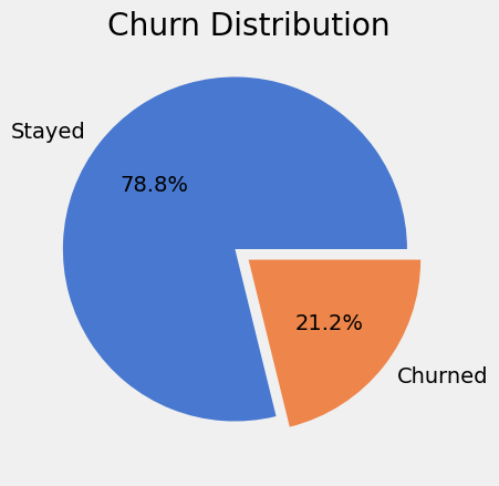
We see that this is a slightly imbalanced dataset with our target class making up ~21.2% of the samples.

cat_cols

Index(['Surname', 'Geography', 'Gender'], dtype='object')

for col in cat_cols:
    if col == 'Surname':
        continue
    xtab = pd.crosstab(df[col], df['Exited'], normalize='index')
    xtab.plot(kind='bar', stacked=True, fontsize=10).legend(loc='lower right')
    plt.title(f'Percentage Distribution of Churn across {col}')
    plt.tight_layout()
    plt.show()

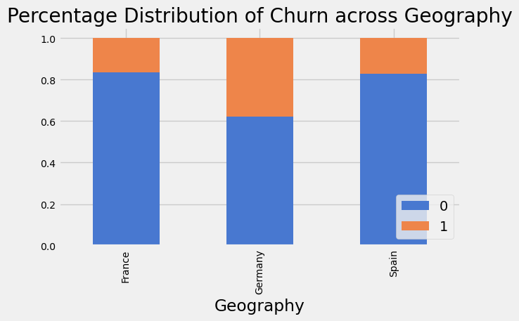
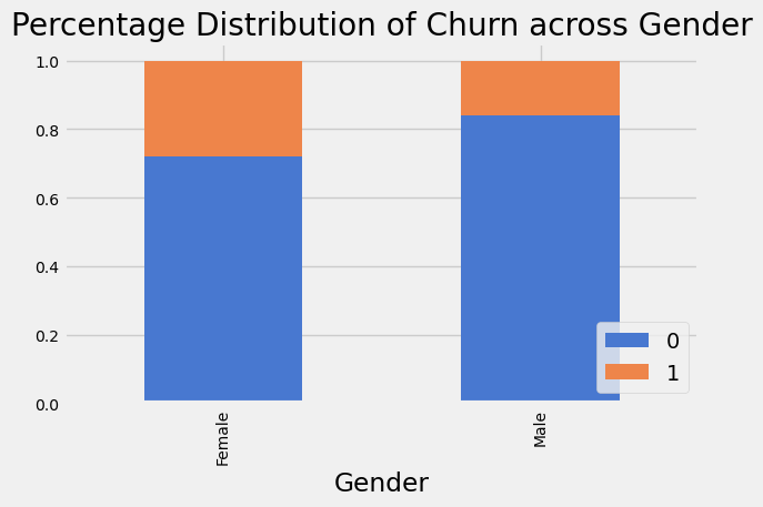
Here we see that a higher proportion of customers from Germany have churned, similar behaviour is seen in Female customers across the dataset. This suggests that the features will be useful in our predictive model.

xtab = pd.crosstab(df['Tenure'], df['Exited'], normalize='index')
xtab.plot(kind='bar', stacked=True, fontsize=10).legend(loc='lower right')
plt.title(f'Percentage Distribution of Churn across Tenure')
plt.tight_layout()
plt.show()

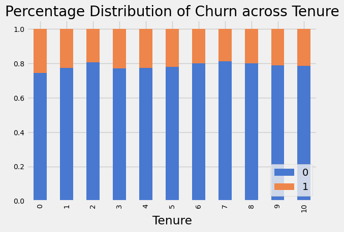
New customer with 0 years with the bank has a slightly higher churn rate than the other customers.

pd.DataFrame(df.groupby(['HasCrCard','IsActiveMember'])[['HasCrCard','IsActiveMember']].value_counts())

		count
HasCrCard	IsActiveMember
0.0	0.0	19646
	1.0	20960
1.0	0.0	63239
	1.0	61189

There is an even distribution among customer that have a credit card and whether they are an active member (unable to verify what this means in the context of this dataset)

In this dataset ~50% of the customers who have a credit card is active, also 50% of the customers who do not have a credit card is active. This goes against the intuition that most customers with an active credit card with the bank will most likely be using it at least occassionally. I suspect this is due to the synthetic nature of the dataset.

In reality more clarity will be required for an ambiguous feature such as IsActiveMember, such as the definition and conditions surrounding a customer being considered active. With these information further feature engineering can possible be conducted to extract more useful information out of this feature.

df.describe()

	id	CustomerId	CreditScore	Age	Tenure	Balance	NumOfProducts	HasCrCard	IsActiveMember	EstimatedSalary	Exited
count	165034.0000	1.650340e+05	165034.000000	165034.000000	165034.000000	165034.000000	165034.000000	165034.000000	165034.000000	165034.000000	165034.000000
mean	82516.5000	1.569201e+07	656.454373	38.125888	5.020353	55478.086689	1.554455	0.753954	0.497770	112574.822734	0.211599
std	47641.3565	7.139782e+04	80.103340	8.867205	2.806159	62817.663278	0.547154	0.430707	0.499997	50292.865585	0.408443
min	0.0000	1.556570e+07	350.000000	18.000000	0.000000	0.000000	1.000000	0.000000	0.000000	11.580000	0.000000
25%	41258.2500	1.563314e+07	597.000000	32.000000	3.000000	0.000000	1.000000	1.000000	0.000000	74637.570000	0.000000
50%	82516.5000	1.569017e+07	659.000000	37.000000	5.000000	0.000000	2.000000	1.000000	0.000000	117948.000000	0.000000
75%	123774.7500	1.575682e+07	710.000000	42.000000	7.000000	119939.517500	2.000000	1.000000	1.000000	155152.467500	0.000000
max	165033.0000	1.581569e+07	850.000000	92.000000	10.000000	250898.090000	4.000000	1.000000	1.000000	199992.480000	1.000000

num_cols

Index(['id', 'CustomerId', 'CreditScore', 'Age', 'Tenure', 'Balance',
       'NumOfProducts', 'HasCrCard', 'IsActiveMember', 'EstimatedSalary',
       'Exited'],
      dtype='object')

for col in num_cols:
    if col in ['id','Exited','HasCrCard','Tenure','NumOfProducts','IsActiveMember']:
        continue
    sns.violinplot(df, x='Exited', y=col)
    plt.title(f'{col} Distribution by Target')
    plt.show()

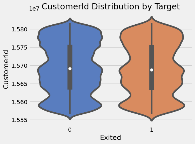
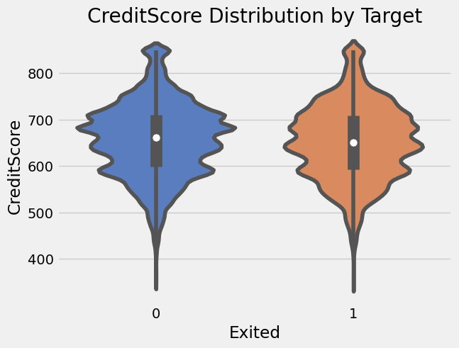
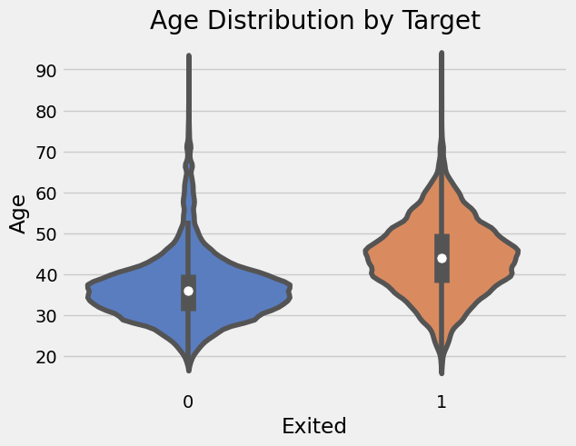
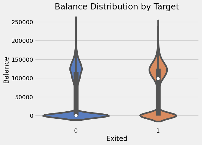
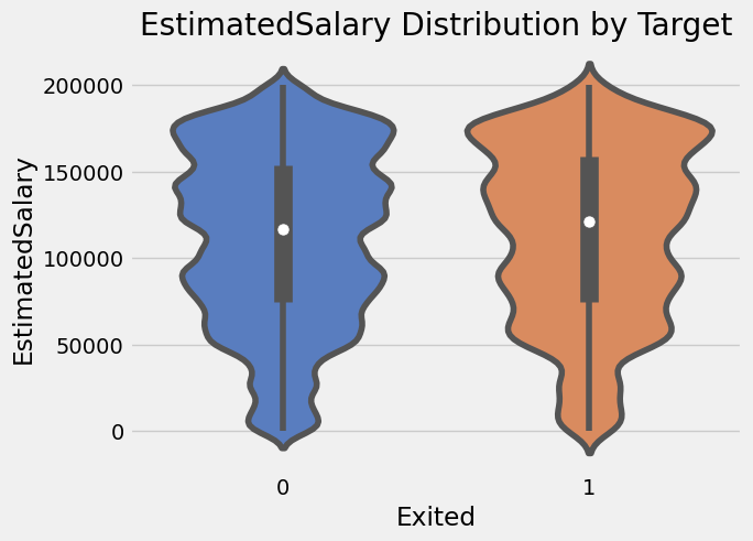
The numerical features all have similar distributions between their churned and non-churned customers except for Age where we see the distribution for churned customers is centred around an older age. (~45 years old vs ~35 years old for non-churned).

# Fitting labelencoders with all the labels from train and test dataset so the label mappings are consistent
test_labels = pd.read_csv('test.csv')[['Geography','Gender','Surname']]
set_geo = set(df['Geography']).union(test_labels['Geography'])
set_gender = set(df['Gender']).union(test_labels['Gender'])
set_surname = set(df['Surname']).union(test_labels['Surname'])
le_geo = LabelEncoder()
le_gender = LabelEncoder()
le_surname = LabelEncoder()
le_geo.fit(list(set_geo))
le_gender.fit(list(set_gender))
le_surname.fit(list(set_surname))

# Encoding categorical features
df['Geography'] = le_geo.transform(df['Geography'])
df['Gender'] = le_gender.transform(df['Gender'])
df['Surname'] = le_surname.transform(df['Surname'])
df.head()

	id	CustomerId	Surname	CreditScore	Geography	Gender	Age	Tenure	Balance	NumOfProducts	HasCrCard	IsActiveMember	EstimatedSalary	Exited
0	0	15674932	1992	668	0	1	33.0	3	0.00	2	1.0	0.0	181449.97	0
1	1	15749177	1993	627	0	1	33.0	1	0.00	2	1.0	1.0	49503.50	0
2	2	15694510	1217	678	0	1	40.0	10	0.00	2	1.0	0.0	184866.69	0
3	3	15741417	1341	581	0	1	34.0	2	148882.54	1	1.0	1.0	84560.88	0
4	4	15766172	483	716	2	1	33.0	5	0.00	2	1.0	1.0	15068.83	0

sns.heatmap(df.corr(numeric_only=True))
plt.title('Correlation Heatmap of Features')
plt.show()

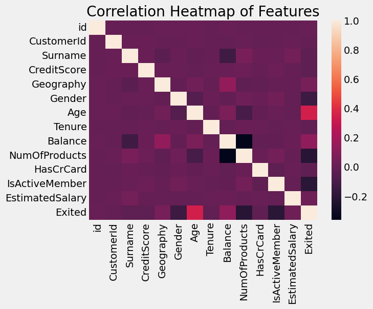
Looking at linear correlation coefficients we see that Age and NumOfProducts have the largest effect on churn

4. Feature Engineering

# Feature engineering
df_eng = df.copy()

# Customer above age of retirement of the 3 countries in dataset
df_eng.loc[df_eng['Age']>=60, 'SeniorAge'] = 1
df_eng.loc[df_eng['Age']<60, 'SeniorAge'] = 0

# Customer is still young
df_eng.loc[df_eng['Age']<=35, 'Young'] = 1
df_eng.loc[df_eng['Age']>35, 'Young'] = 0

# Ratio of Balance and Estimated Salary
df_eng['Ratio_Bal_Sal'] = df_eng['Balance']/df_eng['EstimatedSalary']

# Ratio of Balance and Age
df_eng['Ratio_Bal_Age'] = df_eng['Balance']/df_eng['Age']

# Ratio of Estimated Salary and Age
df_eng['Ratio_Sal_Age'] = df_eng['EstimatedSalary']/df_eng['Age']

# Ratio of Tenure and NumOfProducts
df_eng['Ratio_Ten_Num'] = df_eng['Tenure']/df_eng['NumOfProducts']

# CreditScore bin
df_eng['Bin_CreditScore'] = pd.cut(df_eng['CreditScore'], bins=[0, 600, 700, 900], labels=[0,1,2]).astype(int)

# Age bin
df_eng['Bin_Age'] = df_eng['Age']//10

df_eng.head()

	id	CustomerId	Surname	CreditScore	Geography	Gender	Age	Tenure	Balance	NumOfProducts	...	EstimatedSalary	Exited	SeniorAge	Young	Ratio_Bal_Sal	Ratio_Bal_Age	Ratio_Sal_Age	Ratio_Ten_Num	Bin_CreditScore	Bin_Age
0	0	15674932	1992	668	0	1	33.0	3	0.00	2	...	181449.97	0	0.0	1.0	0.000000	0.000000	5498.483939	1.5	1	3.0
1	1	15749177	1993	627	0	1	33.0	1	0.00	2	...	49503.50	0	0.0	1.0	0.000000	0.000000	1500.106061	0.5	1	3.0
2	2	15694510	1217	678	0	1	40.0	10	0.00	2	...	184866.69	0	0.0	0.0	0.000000	0.000000	4621.667250	5.0	1	4.0
3	3	15741417	1341	581	0	1	34.0	2	148882.54	1	...	84560.88	0	0.0	1.0	1.760655	4378.898235	2487.084706	2.0	0	3.0
4	4	15766172	483	716	2	1	33.0	5	0.00	2	...	15068.83	0	0.0	1.0	0.000000	0.000000	456.631212	2.5	2	3.0

5 rows × 22 columns

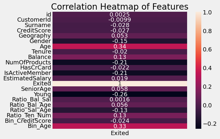
Above are some simple features that were created to transform some of the features to help with our model’s learning. These could be through inspiration and knowledge of the domain or simply random numerical transformations.

df_eng.corr()[['Exited']].index

Index(['id', 'CustomerId', 'Surname', 'CreditScore', 'Geography', 'Gender',
       'Age', 'Tenure', 'Balance', 'NumOfProducts', 'HasCrCard',
       'IsActiveMember', 'EstimatedSalary', 'Exited', 'SeniorAge', 'Young',
       'Ratio_Bal_Sal', 'Ratio_Bal_Age', 'Ratio_Sal_Age', 'Ratio_Ten_Num',
       'Bin_CreditScore', 'Bin_Age'],
      dtype='object')

sns.heatmap(df_eng.corr()[['Exited']], annot=True, yticklabels=df_eng.corr()[['Exited']].index)
plt.title('Correlation Heatmap of Features')
plt.show()

X_train = df_eng.drop(['id','CustomerId','Exited'], axis=1)
X_train.head()

	Surname	CreditScore	Geography	Gender	Age	Tenure	Balance	NumOfProducts	HasCrCard	IsActiveMember	EstimatedSalary	SeniorAge	Young	Ratio_Bal_Sal	Ratio_Bal_Age	Ratio_Sal_Age	Ratio_Ten_Num	Bin_CreditScore	Bin_Age
0	1992	668	0	1	33.0	3	0.00	2	1.0	0.0	181449.97	0.0	1.0	0.000000	0.000000	5498.483939	1.5	1	3.0
1	1993	627	0	1	33.0	1	0.00	2	1.0	1.0	49503.50	0.0	1.0	0.000000	0.000000	1500.106061	0.5	1	3.0
2	1217	678	0	1	40.0	10	0.00	2	1.0	0.0	184866.69	0.0	0.0	0.000000	0.000000	4621.667250	5.0	1	4.0
3	1341	581	0	1	34.0	2	148882.54	1	1.0	1.0	84560.88	0.0	1.0	1.760655	4378.898235	2487.084706	2.0	0	3.0
4	483	716	2	1	33.0	5	0.00	2	1.0	1.0	15068.83	0.0	1.0	0.000000	0.000000	456.631212	2.5	2	3.0

y_train = df_eng['Exited']
y_train.head()

0    0
1    0
2    0
3    0
4    0
Name: Exited, dtype: int64

class AddClustersFeature(BaseEstimator, TransformerMixin):
    def __init__(self, clusters = 8): 
        self.clusters = clusters
        
           
    def fit(self, X, y=None):
        self.X=X
        self.model = KMeans(n_clusters = self.clusters)
        self.model.fit (self.X)
        return self
       
    def transform(self, X):
        self.X=X
        X_=X.copy() # avoiding modification of the original df
        X_ = pd.DataFrame(X_)
        X_['Clusters'] = self.model.predict(X_)
        X_.columns = X_.columns.astype(str)
        #print(X_.info())
        return X_

# Sanity check that function to add cluster as a feature works
cluster_sanity = X_train.copy()
m = AddClustersFeature()
m.fit(cluster_sanity)
cluster_sanity = m.transform(cluster_sanity)
cluster_sanity.head()

	Surname	CreditScore	Geography	Gender	Age	Tenure	Balance	NumOfProducts	HasCrCard	IsActiveMember	EstimatedSalary	SeniorAge	Young	Ratio_Bal_Sal	Ratio_Bal_Age	Ratio_Sal_Age	Ratio_Ten_Num	Bin_CreditScore	Bin_Age	Clusters
0	1992	668	0	1	33.0	3	0.00	2	1.0	0.0	181449.97	0.0	1.0	0.000000	0.000000	5498.483939	1.5	1	3.0	3
1	1993	627	0	1	33.0	1	0.00	2	1.0	1.0	49503.50	0.0	1.0	0.000000	0.000000	1500.106061	0.5	1	3.0	4
2	1217	678	0	1	40.0	10	0.00	2	1.0	0.0	184866.69	0.0	0.0	0.000000	0.000000	4621.667250	5.0	1	4.0	3
3	1341	581	0	1	34.0	2	148882.54	1	1.0	1.0	84560.88	0.0	1.0	1.760655	4378.898235	2487.084706	2.0	0	3.0	7
4	483	716	2	1	33.0	5	0.00	2	1.0	1.0	15068.83	0.0	1.0	0.000000	0.000000	456.631212	2.5	2	3.0	4

Through clustering of our data points, another engineered feature can be added to our dataset. Depending on the clustering algorithm it can provide different additional information about our data points. In this case we are using KMeans which attempts to group similar datapoints based on their Euclidean distances.

5. Modelling

#################################################################

# Instantiate models and params
logreg = LogisticRegression(random_state = 47)
logreg_params = {'C': np.logspace(-4, 4, 6),
                 'solver': ['lbfgs','newton-cg','sag','saga']
                }

rfc = RandomForestClassifier(random_state = 47)
rfc_params = {'n_estimators': [10,50,100],
              'min_samples_split': [2, 5, 10, 20]
             }

xgb = XGBClassifier(random_state = 47,
                    objective='binary:logistic',
                    metric='auc',
                    device = 'cuda', error_score='raise')
xgb_params = {'eta': [0.01,0.1,0.3],
              'max_depth': [3,6,9],
              'lambda': [0.3,0.6,1],
              'alpha': [0,0.1],
              'min_child_weight': [1,10,20],
              'colsample_bytree': [0.25,0.5,1]
             }
              
lgb = LGBMClassifier(random_state = 47,
                    objective='binary',
                    metric='auc',
                    verbosity=-1)
lgb_params = {'max_bin': [10,69,150,255,400],
              'max_depth': [3,6,9],
              'learning_rate': [ 0.01, 0.1],
              'lambda_l1': [0,0.1],
              'lambda_l2': [0,0.3,0.6],
              'num_leaves': [10,31,50]
             }

clfs = [
    ('Logistic Regression', logreg, logreg_params),
    ('Random Forest Classifier', rfc, rfc_params),
    ('XGBoost Classifier', xgb, xgb_params),
    ('LGBM Classifier', lgb, lgb_params)
]

scorers = {
    'accuracy_score': make_scorer(accuracy_score),
    'f1_score': make_scorer(f1_score),
    'roc_auc_score': make_scorer(roc_auc_score)
}

# Compare model performance of (all features) vs (all w/o cluster features) vs (all w/o cluster+surname features) vs (w/o scaling) using xgb
X_train_nosurname = X_train.drop('Surname',axis=1)

pipeline = Pipeline(steps = [
    ('scaler', MinMaxScaler()),
    ('cluster', AddClustersFeature()),
    ('xgb', xgb)
])
pipeline_noclust = Pipeline(steps=[
    ('scaler', MinMaxScaler()),
    ('xgb', xgb)
])
pipeline_noscale = Pipeline(steps=[
    ('cluster', AddClustersFeature()),
    ('xgb', xgb)
])

pipelines = [('Pipeline', pipeline), ('Pipeline_No_Cluster', pipeline_noclust), ('Pipeline_No_Scale', pipeline_noscale)]
results = []
cv = KFold(n_splits=5)
for pipe_name, pipe in pipelines:
    scores = cross_val_score(estimator=pipe, X=X_train, y=y_train, cv=cv, scoring='roc_auc')
    results.append(scores)
    
    scores = cross_val_score(estimator=pipe, X=X_train_nosurname, y=y_train, cv=cv, scoring='roc_auc')
    results.append(scores)

Here we are fitting an XGBoost model in several different scenarios to find our best performing scenario. Below are the scenarios:

1. Dataset is scaled and cluster feature added
2. Dataset is scaled
3. Dataset has cluster feature added This is repeated for training data with and without Surname feature for a total of 6 different scenarios.

best_result = [-1, 0]
for idx, result in enumerate(results):
    mean_result = np.mean(result)
    print(f'Pipeline: {idx}, Mean ROC AUC: {mean_result}')
    if mean_result > best_result[1]:
        best_result = [idx, mean_result]
print(f' Best pipeline is {best_result[0]} with a mean score of {best_result[1]}')
# Best performer is dataset including Surname, with feature scaling and additional cluster feature included

Pipeline: 0, Mean ROC AUC: 0.8888409253562118
Pipeline: 1, Mean ROC AUC: 0.8859394416907461
Pipeline: 2, Mean ROC AUC: 0.8886329403159834
Pipeline: 3, Mean ROC AUC: 0.8858966559943475
Pipeline: 4, Mean ROC AUC: 0.8887585013508655
Pipeline: 5, Mean ROC AUC: 0.8862002696202766
 Best pipeline is 0 with a mean score of 0.8888409253562118

Best performer after 5 fold cross validation is Dataset+Surname feature with feature scaling and cluster feature included. This is the scenario that we will be tuning our final models on.

# Pipeline
results = []
for clf_name, clf, clf_params in clfs:
    gs = GridSearchCV(estimator=clf, 
                      param_grid=clf_params,
                      scoring=scorers,
                      refit='roc_auc_score',
                      verbose=2,
                      error_score='raise'
                     )
    pipeline = Pipeline(steps=[
        ('scaler', MinMaxScaler()),
        ('cluster', AddClustersFeature()),
        ('classifier', gs),
    ])
    pipeline.fit(X_train, y_train)
    result = [clf_name, gs.best_params_, gs.best_score_, gs.cv_results_['mean_test_f1_score'][gs.best_index_], gs.cv_results_['mean_test_accuracy_score'][gs.best_index_]]
    results.append(result)
result_df = pd.DataFrame(results, columns=['Name','Parameters','ROCAUC','F1','Accuracy'])
result_df.head()

Fitting 5 folds for each of 24 candidates, totalling 120 fits
Fitting 5 folds for each of 12 candidates, totalling 60 fits
Fitting 5 folds for each of 486 candidates, totalling 2430 fits
Fitting 5 folds for each of 540 candidates, totalling 2700 fits

	Name	Parameters	ROCAUC	F1	Accuracy
0	Logistic Regression	{'C': 6.309573444801943, 'solver': 'lbfgs'}	0.671971	0.498950	0.833295
1	Random Forest Classifier	{'min_samples_split': 20, 'n_estimators': 100}	0.742522	0.622877	0.863489
2	XGBoost Classifier	{'alpha': 0, 'colsample_bytree': 1, 'eta': 0.3...	0.755960	0.641102	0.866179
3	LGBM Classifier	{'lambda_l1': 0, 'lambda_l2': 0.6, 'learning_r...	0.755667	0.641445	0.866840

Out of the 4 models tuned, XGB and LGBM classifiers have the best performance. As their performance are similar, we shall go one step further and create a final voting classifier to make use of both best performers.

result_df[result_df['Name'].isin(['XGBoost Classifier','LGBM Classifier'])]['Parameters'].tolist()

[{'alpha': 0,
  'colsample_bytree': 1,
  'eta': 0.3,
  'lambda': 0.6,
  'max_depth': 6,
  'min_child_weight': 1},
 {'lambda_l1': 0,
  'lambda_l2': 0.6,
  'learning_rate': 0.1,
  'max_bin': 400,
  'max_depth': 6,
  'num_leaves': 31}]

########################################################################################

xgb = XGBClassifier(random_state = 47,
                    objective='binary:logistic',
                    metric='auc',
                    device = 'cuda',
                    alpha= 0,
                    colsample_bytree= 1,
                    eta= 0.3,
                    reg_lambda= 0.6,
                    max_depth= 6,
                    min_child_weight= 1,
                    error_score='raise')
              
lgb = LGBMClassifier(random_state = 47,
                    objective='binary',
                    metric='auc',
                    verbosity=-1,
                    lambda_l1= 0,
                    lambda_l2= 0.6,
                    learning_rate= 0.1,
                    max_bin= 400,
                    max_depth= 6,
                    num_leaves= 31)

vc = VotingClassifier(estimators=[('xgb',xgb),('lgb',lgb)], voting='soft')

X_train.head()

	Surname	CreditScore	Geography	Gender	Age	Tenure	Balance	NumOfProducts	HasCrCard	IsActiveMember	EstimatedSalary	SeniorAge	Young	Ratio_Bal_Sal	Ratio_Bal_Age	Ratio_Sal_Age	Ratio_Ten_Num	Bin_CreditScore	Bin_Age
0	1992	668	0	1	33.0	3	0.00	2	1.0	0.0	181449.97	0.0	1.0	0.000000	0.000000	5498.483939	1.5	1	3.0
1	1993	627	0	1	33.0	1	0.00	2	1.0	1.0	49503.50	0.0	1.0	0.000000	0.000000	1500.106061	0.5	1	3.0
2	1217	678	0	1	40.0	10	0.00	2	1.0	0.0	184866.69	0.0	0.0	0.000000	0.000000	4621.667250	5.0	1	4.0
3	1341	581	0	1	34.0	2	148882.54	1	1.0	1.0	84560.88	0.0	1.0	1.760655	4378.898235	2487.084706	2.0	0	3.0
4	483	716	2	1	33.0	5	0.00	2	1.0	1.0	15068.83	0.0	1.0	0.000000	0.000000	456.631212	2.5	2	3.0

# Scaling and adding cluster on full training data
scaler = MinMaxScaler()
X_train_final = X_train.copy()
X_train_final = scaler.fit_transform(X_train_final)
X_train_final = AddClustersFeature().fit_transform(X_train_final)
X_train_final

	0	1	2	3	4	5	6	7	8	9	10	11	12	13	14	15	16	17	18	Clusters
0	0.689751	0.636	0.0	1.0	0.202703	0.3	0.000000	0.333333	1.0	0.0	0.907279	0.0	1.0	0.000000	0.000000	0.496366	0.15	0.5	0.250	6
1	0.690097	0.554	0.0	1.0	0.202703	0.1	0.000000	0.333333	1.0	1.0	0.247483	0.0	1.0	0.000000	0.000000	0.135405	0.05	0.5	0.250	3
2	0.421399	0.656	0.0	1.0	0.297297	1.0	0.000000	0.333333	1.0	0.0	0.924364	0.0	0.0	0.000000	0.000000	0.417210	0.50	0.5	0.375	0
3	0.464335	0.462	0.0	1.0	0.216216	0.2	0.593398	0.000000	1.0	1.0	0.422787	0.0	1.0	0.000137	0.424012	0.224506	0.20	0.0	0.250	3
4	0.167244	0.732	1.0	1.0	0.202703	0.5	0.000000	0.333333	1.0	1.0	0.075293	0.0	1.0	0.000000	0.000000	0.041203	0.25	1.0	0.250	3
...	...	...	...	...	...	...	...	...	...	...	...	...	...	...	...	...	...	...	...	...
165029	0.608726	0.634	1.0	0.0	0.202703	0.2	0.000000	0.000000	1.0	1.0	0.659179	0.0	1.0	0.000000	0.000000	0.360636	0.20	0.5	0.250	1
165030	0.687673	0.884	0.0	1.0	0.229730	0.3	0.000000	0.000000	0.0	0.0	0.659177	0.0	1.0	0.000000	0.000000	0.340026	0.30	1.0	0.250	6
165031	0.419321	0.430	0.0	1.0	0.175676	0.5	0.000000	0.000000	1.0	1.0	0.637151	0.0	1.0	0.000000	0.000000	0.371075	0.50	0.0	0.250	3
165032	0.420706	0.408	1.0	0.0	0.162162	0.7	0.643819	0.000000	0.0	1.0	0.355841	0.0	1.0	0.000176	0.521378	0.214156	0.70	0.0	0.250	1
165033	0.916898	1.000	0.0	1.0	0.175676	0.1	0.000000	0.000000	1.0	0.0	0.307880	0.0	1.0	0.000000	0.000000	0.179316	0.10	1.0	0.250	6

165034 rows × 20 columns

cross_val_score(vc, X_train_final, y_train, scoring='roc_auc')

array([0.8940815 , 0.88922709, 0.89204022, 0.89081926, 0.8903584 ])

Above shows our expected model performance if our model did not overfit and trainin/test data share similar distributions

vc.fit(X_train_final, y_train)

VotingClassifier(estimators=[('xgb',
                              XGBClassifier(alpha=0, base_score=None,
                                            booster=None, callbacks=None,
                                            colsample_bylevel=None,
                                            colsample_bynode=None,
                                            colsample_bytree=1, device='cuda',
                                            early_stopping_rounds=None,
                                            enable_categorical=False,
                                            error_score='raise', eta=0.3,
                                            eval_metric=None,
                                            feature_types=None, gamma=None,
                                            grow_policy=None,
                                            importance_type=None,
                                            inter...
                                            learning_rate=None, max_bin=None,
                                            max_cat_threshold=None,
                                            max_cat_to_onehot=None,
                                            max_delta_step=None, max_depth=6,
                                            max_leaves=None, metric='auc',
                                            min_child_weight=1, missing=nan,
                                            monotone_constraints=None,
                                            multi_strategy=None, ...)),
                             ('lgb',
                              LGBMClassifier(lambda_l1=0, lambda_l2=0.6,
                                             max_bin=400, max_depth=6,
                                             metric='auc', objective='binary',
                                             random_state=47, verbosity=-1))],
                 voting='soft')

In a Jupyter environment, please rerun this cell to show the HTML representation or trust the notebook.
On GitHub, the HTML representation is unable to render, please try loading this page with nbviewer.org.

# Preparing test data for prediction
test_df = pd.read_csv('test.csv')
test_df.head()

	id	CustomerId	Surname	CreditScore	Geography	Gender	Age	Tenure	Balance	NumOfProducts	HasCrCard	IsActiveMember	EstimatedSalary
0	165034	15773898	Lucchese	586	France	Female	23.0	2	0.00	2	0.0	1.0	160976.75
1	165035	15782418	Nott	683	France	Female	46.0	2	0.00	1	1.0	0.0	72549.27
2	165036	15807120	K?	656	France	Female	34.0	7	0.00	2	1.0	0.0	138882.09
3	165037	15808905	O'Donnell	681	France	Male	36.0	8	0.00	1	1.0	0.0	113931.57
4	165038	15607314	Higgins	752	Germany	Male	38.0	10	121263.62	1	1.0	0.0	139431.00

test_df.shape

(110023, 13)

test_df['Geography'].unique()

array(['France', 'Germany', 'Spain'], dtype=object)

X_train_final.shape

(165034, 20)

# Encoding categorical features
test_df['Geography'] = le_geo.transform(test_df['Geography'])
test_df['Gender'] = le_gender.transform(test_df['Gender'])
test_df['Surname'] = le_surname.transform(test_df['Surname'])
test_df.head()

# Customer above age of retirement of the 3 countries in dataset
test_df.loc[test_df['Age']>=60, 'SeniorAge'] = 1
test_df.loc[test_df['Age']<60, 'SeniorAge'] = 0

# Customer is still young
test_df.loc[test_df['Age']<=35, 'Young'] = 1
test_df.loc[test_df['Age']>35, 'Young'] = 0

# Ratio of Balance and Estimated Salary
test_df['Ratio_Bal_Sal'] = test_df['Balance']/test_df['EstimatedSalary']

# Ratio of Balance and Age
test_df['Ratio_Bal_Age'] = test_df['Balance']/test_df['Age']

# Ratio of Estimated Salary and Age
test_df['Ratio_Sal_Age'] = test_df['EstimatedSalary']/test_df['Age']

# Ratio of Tenure and NumOfProducts
test_df['Ratio_Ten_Num'] = test_df['Tenure']/test_df['NumOfProducts']

# CreditScore bin
test_df['Bin_CreditScore'] = pd.cut(test_df['CreditScore'], bins=[0, 600, 700, 900], labels=[0,1,2]).astype(int)

# Age bin
test_df['Bin_Age'] = test_df['Age']//10

# Save id to join with final predictions
idx =  test_df['id']

X_test = test_df.drop(['id','CustomerId'], axis=1)

# Scale features and add clusters
X_test = scaler.transform(X_test)
X_test = m.transform(X_test)
X_test.head()

	0	1	2	3	4	5	6	7	8	9	10	11	12	13	14	15	16	17	18	Clusters
0	0.547438	0.472	0.0	0.0	0.067568	0.2	0.000000	0.333333	0.0	1.0	0.804903	0.0	1.0	0.000000	0.000000	0.631827	0.10	0.0	0.125	4
1	0.670014	0.666	0.0	0.0	0.378378	0.2	0.000000	0.000000	1.0	0.0	0.362723	0.0	0.0	0.000000	0.000000	0.142361	0.20	0.5	0.375	4
2	0.460873	0.612	0.0	0.0	0.216216	0.7	0.000000	0.333333	1.0	0.0	0.694419	0.0	1.0	0.000000	0.000000	0.368740	0.35	0.5	0.250	4
3	0.676939	0.662	0.0	1.0	0.243243	0.8	0.000000	0.000000	1.0	0.0	0.569654	0.0	0.0	0.000000	0.000000	0.285685	0.80	0.5	0.250	4
4	0.399238	0.804	0.5	1.0	0.270270	1.0	0.483318	0.000000	1.0	0.0	0.697164	0.0	0.0	0.000068	0.309001	0.331227	1.00	1.0	0.250	4

# Make and export predictions in format for submission
y_pred = vc.predict_proba(X_test)[:, 1]
predictions = pd.concat([idx, pd.Series(y_pred)], axis=1)
predictions.columns = 'id','Exited'
predictions.to_csv('predictions_.csv', index=False)
predictions

	id	Exited
0	165034	0.043242
1	165035	0.856776
2	165036	0.027904
3	165037	0.242382
4	165038	0.358144
...	...	...
110018	275052	0.030970
110019	275053	0.154990
110020	275054	0.023756
110021	275055	0.160589
110022	275056	0.196556

110023 rows × 2 columns

Our predictions currently has a public score of 0.88895 after submission, which is close to what we have expected.

6. Conclusion

In this notebook we have explored a synthetic bank churn dataset and briefly discussed what could be done differently in a real world scenario. With a churn rate of ~21% our model has an ROCAUC of 0.88895 which appears to be a relatively good performance that beats out a random guess strategy. With some domain knowledge or time investment, one can create certain conditional strategies that predicts customer churn. Further analysis between the predictive model and those conditional strategies will then tell us if the model performance is indeed worthwhile.