Multi-Class Prediction of Obesity Risk

Contents
1. Introduction
In this notebook we take a look at a Kaggle Playground Series competition where users submit their predictions for a multi-class classification problem on the sample’s weight class.
2. Data Cleaning
import pandas as pd
import numpy as np
import matplotlib.pyplot as plt
import seaborn as sns

from sklearn.preprocessing import MinMaxScaler
from sklearn.model_selection import train_test_split, GridSearchCV
from sklearn.linear_model import LogisticRegression
from sklearn.ensemble import RandomForestClassifier
from xgboost import XGBClassifier
from lightgbm import LGBMClassifier

from sklearn.pipeline import Pipeline
from sklearn.metrics import classification_report, confusion_matrix, accuracy_score, f1_score, auc, roc_curve, roc_auc_score, make_scorer
import warnings
warnings.filterwarnings('ignore')
# Data import and cleaning
data = pd.read_csv('train.csv')
data.head()
| id | Gender | Age | Height | Weight | family_history_with_overweight | FAVC | FCVC | NCP | CAEC | SMOKE | CH2O | SCC | FAF | TUE | CALC | MTRANS | NObeyesdad | |
|---|---|---|---|---|---|---|---|---|---|---|---|---|---|---|---|---|---|---|
| 0 | 0 | Male | 24.443011 | 1.699998 | 81.669950 | yes | yes | 2.000000 | 2.983297 | Sometimes | no | 2.763573 | no | 0.000000 | 0.976473 | Sometimes | Public_Transportation | Overweight_Level_II |
| 1 | 1 | Female | 18.000000 | 1.560000 | 57.000000 | yes | yes | 2.000000 | 3.000000 | Frequently | no | 2.000000 | no | 1.000000 | 1.000000 | no | Automobile | Normal_Weight |
| 2 | 2 | Female | 18.000000 | 1.711460 | 50.165754 | yes | yes | 1.880534 | 1.411685 | Sometimes | no | 1.910378 | no | 0.866045 | 1.673584 | no | Public_Transportation | Insufficient_Weight |
| 3 | 3 | Female | 20.952737 | 1.710730 | 131.274851 | yes | yes | 3.000000 | 3.000000 | Sometimes | no | 1.674061 | no | 1.467863 | 0.780199 | Sometimes | Public_Transportation | Obesity_Type_III |
| 4 | 4 | Male | 31.641081 | 1.914186 | 93.798055 | yes | yes | 2.679664 | 1.971472 | Sometimes | no | 1.979848 | no | 1.967973 | 0.931721 | Sometimes | Public_Transportation | Overweight_Level_II |
Descriptions of the columns within the dataset:
- Frequent consumption of high caloric food (FAVC)
- Frequency of consumption of vegetables (FCVC)
- Number of main meals (NCP)
- Consumption of food between meals (CAEC)
- Consumption of water daily (CH20)
- and Consumption of alcohol (CALC)
- The attributes related with the physical condition are: Calories consumption monitoring (SCC)
- Physical activity frequency (FAF)
- Time using technology devices (TUE)
- Transportation used (MTRANS)
data.info()
<class 'pandas.core.frame.DataFrame'>
RangeIndex: 20758 entries, 0 to 20757
Data columns (total 18 columns):
 #   Column                          Non-Null Count  Dtype
---  ------                          --------------  -----
 0   id                              20758 non-null  int64
 1   Gender                          20758 non-null  object
 2   Age                             20758 non-null  float64
 3   Height                          20758 non-null  float64
 4   Weight                          20758 non-null  float64
 5   family_history_with_overweight  20758 non-null  object
 6   FAVC                            20758 non-null  object
 7   FCVC                            20758 non-null  float64
 8   NCP                             20758 non-null  float64
 9   CAEC                            20758 non-null  object
 10  SMOKE                           20758 non-null  object
 11  CH2O                            20758 non-null  float64
 12  SCC                             20758 non-null  object
 13  FAF                             20758 non-null  float64
 14  TUE                             20758 non-null  float64
 15  CALC                            20758 non-null  object
 16  MTRANS                          20758 non-null  object
 17  NObeyesdad                      20758 non-null  object
dtypes: float64(8), int64(1), object(9)
memory usage: 2.9+ MB


'\nFrequent consumption of high caloric food (FAVC)\nFrequency of consumption of vegetables (FCVC)\nNumber of main meals (NCP)\nConsumption of food between meals (CAEC)\nConsumption of water daily (CH20)\nand Consumption of alcohol (CALC)\nThe attributes related with the physical condition are: Calories consumption monitoring (SCC)\nPhysical activity frequency (FAF)\nTime using technology devices (TUE)\nTransportation used (MTRANS)\n'
data = data.drop('id',axis=1)
data.head()
| Gender | Age | Height | Weight | family_history_with_overweight | FAVC | FCVC | NCP | CAEC | SMOKE | CH2O | SCC | FAF | TUE | CALC | MTRANS | NObeyesdad | |
|---|---|---|---|---|---|---|---|---|---|---|---|---|---|---|---|---|---|
| 0 | Male | 24.443011 | 1.699998 | 81.669950 | yes | yes | 2.000000 | 2.983297 | Sometimes | no | 2.763573 | no | 0.000000 | 0.976473 | Sometimes | Public_Transportation | Overweight_Level_II |
| 1 | Female | 18.000000 | 1.560000 | 57.000000 | yes | yes | 2.000000 | 3.000000 | Frequently | no | 2.000000 | no | 1.000000 | 1.000000 | no | Automobile | Normal_Weight |
| 2 | Female | 18.000000 | 1.711460 | 50.165754 | yes | yes | 1.880534 | 1.411685 | Sometimes | no | 1.910378 | no | 0.866045 | 1.673584 | no | Public_Transportation | Insufficient_Weight |
| 3 | Female | 20.952737 | 1.710730 | 131.274851 | yes | yes | 3.000000 | 3.000000 | Sometimes | no | 1.674061 | no | 1.467863 | 0.780199 | Sometimes | Public_Transportation | Obesity_Type_III |
| 4 | Male | 31.641081 | 1.914186 | 93.798055 | yes | yes | 2.679664 | 1.971472 | Sometimes | no | 1.979848 | no | 1.967973 | 0.931721 | Sometimes | Public_Transportation | Overweight_Level_II |
data.shape
(20758, 17)
data.duplicated().sum()
0
data.isna().sum()
Gender                            0
Age                               0
Height                            0
Weight                            0
family_history_with_overweight    0
FAVC                              0
FCVC                              0
NCP                               0
CAEC                              0
SMOKE                             0
CH2O                              0
SCC                               0
FAF                               0
TUE                               0
CALC                              0
MTRANS                            0
NObeyesdad                        0
dtype: int64
3. Exploration and Visualization
data.describe()
| Age | Height | Weight | FCVC | NCP | CH2O | FAF | TUE | |
|---|---|---|---|---|---|---|---|---|
| count | 20758.000000 | 20758.000000 | 20758.000000 | 20758.000000 | 20758.000000 | 20758.000000 | 20758.000000 | 20758.000000 |
| mean | 23.841804 | 1.700245 | 87.887768 | 2.445908 | 2.761332 | 2.029418 | 0.981747 | 0.616756 |
| std | 5.688072 | 0.087312 | 26.379443 | 0.533218 | 0.705375 | 0.608467 | 0.838302 | 0.602113 |
| min | 14.000000 | 1.450000 | 39.000000 | 1.000000 | 1.000000 | 1.000000 | 0.000000 | 0.000000 |
| 25% | 20.000000 | 1.631856 | 66.000000 | 2.000000 | 3.000000 | 1.792022 | 0.008013 | 0.000000 |
| 50% | 22.815416 | 1.700000 | 84.064875 | 2.393837 | 3.000000 | 2.000000 | 1.000000 | 0.573887 |
| 75% | 26.000000 | 1.762887 | 111.600553 | 3.000000 | 3.000000 | 2.549617 | 1.587406 | 1.000000 |
| max | 61.000000 | 1.975663 | 165.057269 | 3.000000 | 4.000000 | 3.000000 | 3.000000 | 2.000000 |
num_cols = data.select_dtypes(exclude=['object']).columns
for col in data.select_dtypes('object').columns:
    print(data[col].value_counts())
    print("---------------\n")
Gender
Female    10422
Male      10336
Name: count, dtype: int64
---------------

family_history_with_overweight
yes    17014
no      3744
Name: count, dtype: int64
---------------

FAVC
yes    18982
no      1776
Name: count, dtype: int64
---------------

CAEC
Sometimes     17529
Frequently     2472
Always          478
no              279
Name: count, dtype: int64
---------------

SMOKE
no     20513
yes      245
Name: count, dtype: int64
---------------

SCC
no     20071
yes      687
Name: count, dtype: int64
---------------

CALC
Sometimes     15066
no             5163
Frequently      529
Name: count, dtype: int64
---------------

MTRANS
Public_Transportation    16687
Automobile                3534
Walking                    467
Motorbike                   38
Bike                        32
Name: count, dtype: int64
---------------

NObeyesdad
Obesity_Type_III       4046
Obesity_Type_II        3248
Normal_Weight          3082
Obesity_Type_I         2910
Insufficient_Weight    2523
Overweight_Level_II    2522
Overweight_Level_I     2427
Name: count, dtype: int64
---------------
We see that there are some ordinal data
- Consumption of food between meals (CAEC)
- Consumption of alcohol (CALC)
and some nominal data
- Transportation used (MTRANS)
later in the notebook we will encode these categorical features using different techniques to account for the ordinality.
"""
•Underweight Less than 18.5
•Normal 18.5 to 24.9
•Overweight 25.0 to 29.9
•Obesity I 30.0 to 34.9
•Obesity II 35.0 to 39.9
•Obesity III Higher than 40
"""
'\n•Underweight Less than 18.5\n•Normal 18.5 to 24.9\n•Overweight 25.0 to 29.9\n•Obesity I 30.0 to 34.9\n•Obesity II 35.0 to 39.9\n•Obesity III Higher than 40\n'
sns.countplot(data=data, x='NObeyesdad', hue='Gender', order=['Insufficient_Weight','Normal_Weight','Overweight_Level_I','Overweight_Level_II','Obesity_Type_I','Obesity_Type_II','Obesity_Type_III'])
plt.xticks(rotation=45, horizontalalignment='right')
plt.title("Target class by Gender")
plt.tight_layout()
plt.show()
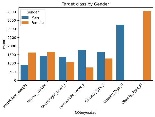
Looking at the distribution of weightclass by gender we see that Obesity Type II is almost entirely made up of Male samples and Obesity Type III is almost entirely made up of Female samples.
This can be attributed to the synthetic nature of the dataset, and assuming that the test data will be generated with the same distribution this should not impact the performance of our model.
sns.histplot(data=data, x='Age', hue='Gender', log_scale=(False,True))
plt.title("Distribution of samples by Age and Gender")
plt.show() # Most samples are between 20~40 years old
C:\Users\wenhao\anaconda3\envs\ML\Lib\site-packages\seaborn\_oldcore.py:1119: FutureWarning: use_inf_as_na option is deprecated and will be removed in a future version. Convert inf values to NaN before operating instead.
  with pd.option_context('mode.use_inf_as_na', True):
C:\Users\wenhao\anaconda3\envs\ML\Lib\site-packages\seaborn\_oldcore.py:1075: FutureWarning: When grouping with a length-1 list-like, you will need to pass a length-1 tuple to get_group in a future version of pandas. Pass `(name,)` instead of `name` to silence this warning.
  data_subset = grouped_data.get_group(pd_key)
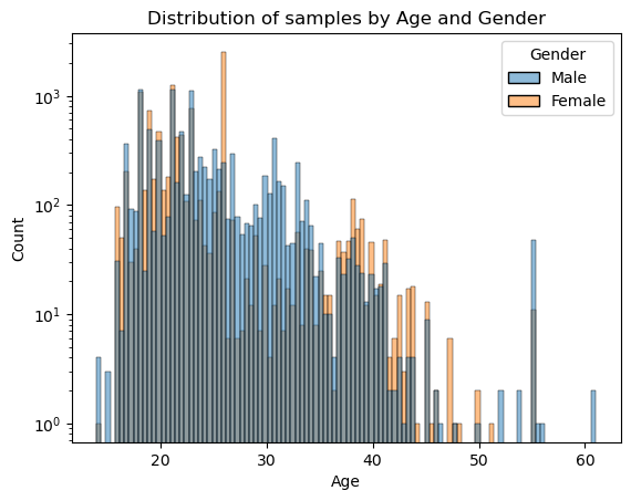
We see most samples fall between 20 ~ 40 years old, take note that this y axis is in log scale making it look more uniform than it really is.
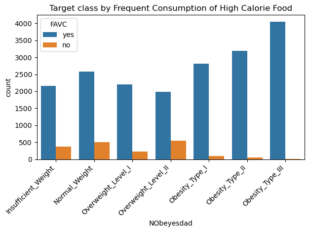
sns.countplot(data=data, x='NObeyesdad', hue='FAVC', order=['Insufficient_Weight','Normal_Weight','Overweight_Level_I','Overweight_Level_II','Obesity_Type_I','Obesity_Type_II','Obesity_Type_III'])
plt.xticks(rotation=45, horizontalalignment='right')
plt.title("Target class by Frequent Consumption of High Calorie Food")
plt.tight_layout()
plt.show() # Different CAEC distribution for target classes, almost all obese samples falls under "Sometimes" category.
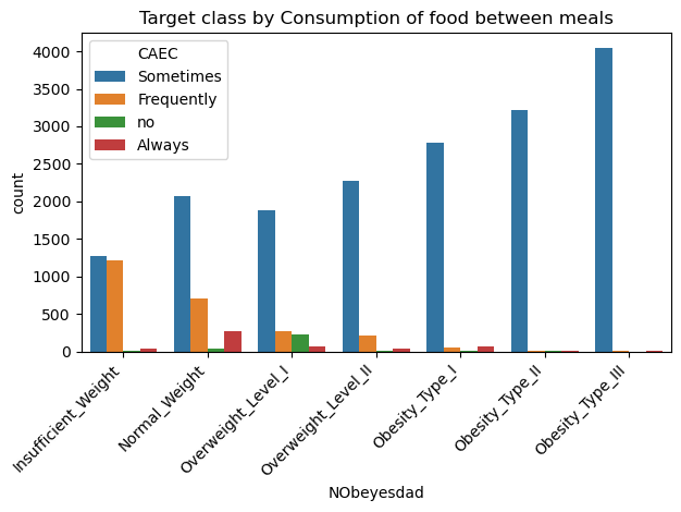
sns.countplot(data=data, x='NObeyesdad', hue='CAEC', order=['Insufficient_Weight','Normal_Weight','Overweight_Level_I','Overweight_Level_II','Obesity_Type_I','Obesity_Type_II','Obesity_Type_III'])
plt.xticks(rotation=45, horizontalalignment='right')
plt.title("Target class by Consumption of food between meals")
plt.tight_layout()
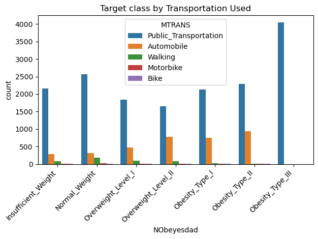
plt.show() # Almost no obese samples fall under Walking/Motorbike/Bike
sns.countplot(data=data, x='NObeyesdad', hue='MTRANS', order=['Insufficient_Weight','Normal_Weight','Overweight_Level_I','Overweight_Level_II','Obesity_Type_I','Obesity_Type_II','Obesity_Type_III'])
plt.xticks(rotation=45, horizontalalignment='right')
plt.title("Target class by Transportation Used")
plt.tight_layout()
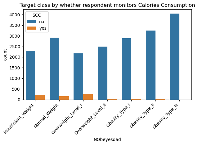
plt.show() # Almost no obese sample monitor their calories consumption
sns.countplot(data=data, x='NObeyesdad', hue='SCC', order=['Insufficient_Weight','Normal_Weight','Overweight_Level_I','Overweight_Level_II','Obesity_Type_I','Obesity_Type_II','Obesity_Type_III'])
plt.xticks(rotation=45, horizontalalignment='right')
plt.title("Target class by whether respondent monitors Calories Consumption")
plt.tight_layout()
plt.show()
# Feature encoding
"""
Ordinal encode
Consumption of food between meals (CAEC)
Consumption of alcohol (CALC)
Target columns (NObeyesdad)

Nominal encode
Transportation used (MTRANS)
"""
'\nOrdinal encode\nConsumption of food between meals (CAEC)\nConsumption of alcohol (CALC)\nTarget columns (NObeyesdad)\n\nNominal encode\nTransportation used (MTRANS)\n'
data.select_dtypes('object').columns
Index(['Gender', 'family_history_with_overweight', 'FAVC', 'CAEC', 'SMOKE',
       'SCC', 'CALC', 'MTRANS', 'NObeyesdad'],
      dtype='object')
# Dummy encoding
dummy_cols = ['Gender', 'family_history_with_overweight', 'FAVC', 'SMOKE',
       'SCC', 'MTRANS']
dummy_var = pd.get_dummies(data[dummy_cols], drop_first=True, dtype=int)
dummy_var.head()
| Gender_Male | family_history_with_overweight_yes | FAVC_yes | SMOKE_yes | SCC_yes | MTRANS_Bike | MTRANS_Motorbike | MTRANS_Public_Transportation | MTRANS_Walking | |
|---|---|---|---|---|---|---|---|---|---|
| 0 | 1 | 1 | 1 | 0 | 0 | 0 | 0 | 1 | 0 |
| 1 | 0 | 1 | 1 | 0 | 0 | 0 | 0 | 0 | 0 |
| 2 | 0 | 1 | 1 | 0 | 0 | 0 | 0 | 1 | 0 |
| 3 | 0 | 1 | 1 | 0 | 0 | 0 | 0 | 1 | 0 |
| 4 | 1 | 1 | 1 | 0 | 0 | 0 | 0 | 1 | 0 |
data = pd.concat([data, dummy_var], axis=1)
data = data.drop(dummy_cols,axis=1)
data.head()
| Age | Height | Weight | FCVC | NCP | CAEC | CH2O | FAF | TUE | CALC | NObeyesdad | Gender_Male | family_history_with_overweight_yes | FAVC_yes | SMOKE_yes | SCC_yes | MTRANS_Bike | MTRANS_Motorbike | MTRANS_Public_Transportation | MTRANS_Walking | |
|---|---|---|---|---|---|---|---|---|---|---|---|---|---|---|---|---|---|---|---|---|
| 0 | 24.443011 | 1.699998 | 81.669950 | 2.000000 | 2.983297 | Sometimes | 2.763573 | 0.000000 | 0.976473 | Sometimes | Overweight_Level_II | 1 | 1 | 1 | 0 | 0 | 0 | 0 | 1 | 0 |
| 1 | 18.000000 | 1.560000 | 57.000000 | 2.000000 | 3.000000 | Frequently | 2.000000 | 1.000000 | 1.000000 | no | Normal_Weight | 0 | 1 | 1 | 0 | 0 | 0 | 0 | 0 | 0 |
| 2 | 18.000000 | 1.711460 | 50.165754 | 1.880534 | 1.411685 | Sometimes | 1.910378 | 0.866045 | 1.673584 | no | Insufficient_Weight | 0 | 1 | 1 | 0 | 0 | 0 | 0 | 1 | 0 |
| 3 | 20.952737 | 1.710730 | 131.274851 | 3.000000 | 3.000000 | Sometimes | 1.674061 | 1.467863 | 0.780199 | Sometimes | Obesity_Type_III | 0 | 1 | 1 | 0 | 0 | 0 | 0 | 1 | 0 |
| 4 | 31.641081 | 1.914186 | 93.798055 | 2.679664 | 1.971472 | Sometimes | 1.979848 | 1.967973 | 0.931721 | Sometimes | Overweight_Level_II | 1 | 1 | 1 | 0 | 0 | 0 | 0 | 1 | 0 |
# Ordinal encoding
for col in ['CAEC','CALC','NObeyesdad']:
    print(data[col].unique())
['Sometimes' 'Frequently' 'no' 'Always']
['Sometimes' 'no' 'Frequently']
['Overweight_Level_II' 'Normal_Weight' 'Insufficient_Weight'
 'Obesity_Type_III' 'Obesity_Type_II' 'Overweight_Level_I'
 'Obesity_Type_I']
data['CAEC'] = data['CAEC'].map({'no':0,'Sometimes':1,'Frequently':2,'Always':3})
data['CALC'] = data['CALC'].map({'no':0,'Sometimes':1,'Frequently':2})
data['NObeyesdad'] = data['NObeyesdad'].map({'Insufficient_Weight':0,'Normal_Weight':1,'Overweight_Level_I':2,'Overweight_Level_II':3,'Obesity_Type_I':4,'Obesity_Type_II':5,'Obesity_Type_III':6})
data[['CAEC','CALC','NObeyesdad']].head()
| CAEC | CALC | NObeyesdad | |
|---|---|---|---|
| 0 | 1 | 1 | 3 |
| 1 | 2 | 0 | 1 |
| 2 | 1 | 0 | 0 |
| 3 | 1 | 1 | 6 |
| 4 | 1 | 1 | 3 |
The dataset has been cleaned and encoded, before moving on to modelling we will create a few new features to help provide more information to our predictive model.
Feature Engineering
# Feature engineering
data_eng = data.copy()
data_eng[['Height','Weight']].describe() # Looks like metric unit
| Height | Weight | |
|---|---|---|
| count | 20758.000000 | 20758.000000 |
| mean | 1.700245 | 87.887768 |
| std | 0.087312 | 26.379443 |
| min | 1.450000 | 39.000000 |
| 25% | 1.631856 | 66.000000 |
| 50% | 1.700000 | 84.064875 |
| 75% | 1.762887 | 111.600553 |
| max | 1.975663 | 165.057269 |
data_eng['bmi'] = data_eng['Weight'] / (data_eng['Height'] ** 2)
data_eng[['Height','Weight','bmi']].head()
| Height | Weight | bmi | |
|---|---|---|---|
| 0 | 1.699998 | 81.669950 | 28.259565 |
| 1 | 1.560000 | 57.000000 | 23.422091 |
| 2 | 1.711460 | 50.165754 | 17.126706 |
| 3 | 1.710730 | 131.274851 | 44.855798 |
| 4 | 1.914186 | 93.798055 | 25.599151 |
data_eng[['NCP','FCVC']].describe()
| NCP | FCVC | |
|---|---|---|
| count | 20758.000000 | 20758.000000 |
| mean | 2.761332 | 2.445908 |
| std | 0.705375 | 0.533218 |
| min | 1.000000 | 1.000000 |
| 25% | 3.000000 | 2.000000 |
| 50% | 3.000000 | 2.393837 |
| 75% | 3.000000 | 3.000000 |
| max | 4.000000 | 3.000000 |
data_eng['veg_meal_ratio'] = data_eng['FCVC']/data_eng['NCP']
data_eng[['NCP','FCVC','veg_meal_ratio']].head()
| NCP | FCVC | veg_meal_ratio | |
|---|---|---|---|
| 0 | 2.983297 | 2.000000 | 0.670399 |
| 1 | 3.000000 | 2.000000 | 0.666667 |
| 2 | 1.411685 | 1.880534 | 1.332120 |
| 3 | 3.000000 | 3.000000 | 1.000000 |
| 4 | 1.971472 | 2.679664 | 1.359220 |
5. Modelling
X_train = data_eng.drop('NObeyesdad',axis=1)
X.head()
| Age | Height | Weight | FCVC | NCP | CAEC | CH2O | FAF | TUE | CALC | ... | family_history_with_overweight_yes | FAVC_yes | SMOKE_yes | SCC_yes | MTRANS_Bike | MTRANS_Motorbike | MTRANS_Public_Transportation | MTRANS_Walking | bmi | veg_meal_ratio | |
|---|---|---|---|---|---|---|---|---|---|---|---|---|---|---|---|---|---|---|---|---|---|
| 0 | 24.443011 | 1.699998 | 81.669950 | 2.000000 | 2.983297 | 1 | 2.763573 | 0.000000 | 0.976473 | 1 | ... | 1 | 1 | 0 | 0 | 0 | 0 | 1 | 0 | 28.259565 | 0.670399 |
| 1 | 18.000000 | 1.560000 | 57.000000 | 2.000000 | 3.000000 | 2 | 2.000000 | 1.000000 | 1.000000 | 0 | ... | 1 | 1 | 0 | 0 | 0 | 0 | 0 | 0 | 23.422091 | 0.666667 |
| 2 | 18.000000 | 1.711460 | 50.165754 | 1.880534 | 1.411685 | 1 | 1.910378 | 0.866045 | 1.673584 | 0 | ... | 1 | 1 | 0 | 0 | 0 | 0 | 1 | 0 | 17.126706 | 1.332120 |
| 3 | 20.952737 | 1.710730 | 131.274851 | 3.000000 | 3.000000 | 1 | 1.674061 | 1.467863 | 0.780199 | 1 | ... | 1 | 1 | 0 | 0 | 0 | 0 | 1 | 0 | 44.855798 | 1.000000 |
| 4 | 31.641081 | 1.914186 | 93.798055 | 2.679664 | 1.971472 | 1 | 1.979848 | 1.967973 | 0.931721 | 1 | ... | 1 | 1 | 0 | 0 | 0 | 0 | 1 | 0 | 25.599151 | 1.359220 |
5 rows × 21 columns
y_train = data_eng['NObeyesdad']
y.head()
0    3
1    1
2    0
3    6
4    3
Name: NObeyesdad, dtype: int64
# Instantitate classifiers and their params
logreg = LogisticRegression(random_state = 47)
logreg_params = {'C': np.logspace(-4, 4, 6),
                 'solver': ['lbfgs','newton-cg','sag','saga'],
                 'multi_class': ['ovr','multinomial']
                }
rfc = RandomForestClassifier(random_state = 47)
rfc_params = {'n_estimators': [10,50,100,250],
              'min_samples_split': [2, 5, 10, 20]
             }
xgb = XGBClassifier(random_state = 47, device = 'gpu')
xgb_params = {'booster': ['gbtree','dart'],
              'eta': [0.01,0.3],
              'max_depth': [3,6,9],
              'lambda': [0.1,1]
             }

lgb = LGBMClassifier(random_state = 47)
lgb_params = {'max_bin': [10,69,150,255,400],
              'learning_rate': [ 0.01, 0.1],
              'num_leaves': [10,31]
             }

clfs = [
    ('Logistic Regression', logreg, logreg_params),
    ('Random Forest Classifier', rfc, rfc_params),
    ('XGBoost Classifier', xgb, xgb_params),
    ('LGBM Classifier', lgb, lgb_params)
]

scorers = {
    'accuracy_score': make_scorer(accuracy_score),
    'f1_score': make_scorer(f1_score, average='micro')
}
# Pipeline
results = []
for clf_name, clf, clf_params in clfs:
    gs = GridSearchCV(estimator=clf,
                      param_grid=clf_params,
                      scoring=scorers,
                      refit='accuracy_score',
                      verbose=1
                     )
    pipeline = Pipeline(steps=[
        ('scaler', MinMaxScaler()),
        ('classifier', gs),
    ])
    pipeline.fit(X, y)
    result = [clf_name, gs.best_params_, gs.best_score_, gs.cv_results_['mean_test_f1_score'][gs.best_index_]]
    results.append(result)
result_df = pd.DataFrame(results, columns=['Name','Parameters','Accuracy','F1'])
result_df.head()
Fitting 5 folds for each of 48 candidates, totalling 240 fits
Fitting 5 folds for each of 16 candidates, totalling 80 fits
Fitting 5 folds for each of 24 candidates, totalling 120 fits
Fitting 5 folds for each of 20 candidates, totalling 100 fits
| Name | Parameters | Accuracy | F1 | |
|---|---|---|---|---|
| 0 | Logistic Regression | {'C': 10000.0, 'multi_class': 'multinomial', '... | 0.866462 | 0.866462 |
| 1 | Random Forest Classifier | {'min_samples_split': 5, 'n_estimators': 250} | 0.901532 | 0.901532 |
| 2 | XGBoost Classifier | {'booster': 'gbtree', 'eta': 0.3, 'lambda': 1,... | 0.906542 | 0.906542 |
| 3 | LGBM Classifier | {'learning_rate': 0.1, 'max_bin': 400, 'num_le... | 0.905723 | 0.905723 |
# Process test data
test_df = pd.read_csv('test.csv')
ids = test_df['id']
test_df = test_df.drop('id', axis=1)
# Nominal Encode
test_dummy_var = pd.get_dummies(test_df[dummy_cols], drop_first=True, dtype=int)
test_df = pd.concat([test_df, test_dummy_var], axis=1)
test_df = test_df.drop(dummy_cols,axis=1)

# Ordinal Encode
test_df['CAEC'] = test_df['CAEC'].map({'no':0,'Sometimes':1,'Frequently':2,'Always':3})
test_df['CALC'] = test_df['CALC'].map({'no':0,'Sometimes':1,'Frequently':2})
#test_df['NObeyesdad'] = test_df['NObeyesdad'].map({'Insufficient_Weight':0,'Normal_Weight':1,'Overweight_Level_I':2,'Overweight_Level_II':3,'Obesity_Type_I':4,'Obesity_Type_II':5,'Obesity_Type_III':6})

# Feature Engineering
test_df['bmi'] = test_df['Weight'] / (test_df['Height'] ** 2)
test_df['veg_meal_ratio'] = test_df['FCVC']/test_df['NCP']

# Feature Scaling (Fit on full training data)
scaler = MinMaxScaler()
train_df[num_cols] = scaler.fit_transform(train_df[num_cols])
test_df[num_cols] = scaler.transform(test_df[num_cols])
test_df.head()
| Age | Height | Weight | FCVC | NCP | CAEC | CH2O | FAF | TUE | CALC | ... | family_history_with_overweight_yes | FAVC_yes | SMOKE_yes | SCC_yes | MTRANS_Bike | MTRANS_Motorbike | MTRANS_Public_Transportation | MTRANS_Walking | bmi | veg_meal_ratio | |
|---|---|---|---|---|---|---|---|---|---|---|---|---|---|---|---|---|---|---|---|---|---|
| 0 | 26.899886 | 1.848294 | 120.644178 | 2.938616 | 3.000000 | 1 | 2.825629 | 0.855400 | 0.000000 | 1.0 | ... | 1 | 1 | 0 | 0 | 0 | 0 | 1 | 0 | 35.315411 | 0.979539 |
| 1 | 21.000000 | 1.600000 | 66.000000 | 2.000000 | 1.000000 | 1 | 3.000000 | 1.000000 | 0.000000 | 1.0 | ... | 1 | 1 | 0 | 0 | 0 | 0 | 1 | 0 | 25.781250 | 2.000000 |
| 2 | 26.000000 | 1.643355 | 111.600553 | 3.000000 | 3.000000 | 1 | 2.621877 | 0.000000 | 0.250502 | 1.0 | ... | 1 | 1 | 0 | 0 | 0 | 0 | 1 | 0 | 41.324115 | 1.000000 |
| 3 | 20.979254 | 1.553127 | 103.669116 | 2.000000 | 2.977909 | 1 | 2.786417 | 0.094851 | 0.000000 | 1.0 | ... | 1 | 1 | 0 | 0 | 0 | 0 | 1 | 0 | 42.976937 | 0.671612 |
| 4 | 26.000000 | 1.627396 | 104.835346 | 3.000000 | 3.000000 | 1 | 2.653531 | 0.000000 | 0.741069 | 1.0 | ... | 1 | 1 | 0 | 0 | 0 | 0 | 1 | 0 | 39.584143 | 1.000000 |
5 rows × 21 columns
# Get best classifier's parameters
print(*zip(result_df[result_df['Name'] == 'XGBoost Classifier']['Parameters']))
({'booster': 'gbtree', 'eta': 0.3, 'lambda': 1, 'max_depth': 3},)
best_clf = XGBClassifier(booster='gbtree', eta=0.3, reg_lambda=1, max_depth=3, random_state=42)
best_clf.fit(X_train, y_train)
y_pred = best_clf.predict(test_df)
# Formatting and mapping predictions for kaggle submission
predictions = pd.concat([ids, pd.Series(y_pred)], axis = 1)
predictions.columns = 'ids','NObeyesdad'
predictions
| ids | NObeyesdad | |
|---|---|---|
| 0 | 20758 | 5 |
| 1 | 20759 | 2 |
| 2 | 20760 | 6 |
| 3 | 20761 | 4 |
| 4 | 20762 | 6 |
| ... | ... | ... |
| 13835 | 34593 | 3 |
| 13836 | 34594 | 1 |
| 13837 | 34595 | 0 |
| 13838 | 34596 | 1 |
| 13839 | 34597 | 5 |
13840 rows × 2 columns
target_map = {'Insufficient_Weight':0,'Normal_Weight':1,'Overweight_Level_I':2,'Overweight_Level_II':3,'Obesity_Type_I':4,'Obesity_Type_II':5,'Obesity_Type_III':6}
target_unmap = {v: k for k, v in target_map.items()}
target_unmap
{0: 'Insufficient_Weight',
 1: 'Normal_Weight',
 2: 'Overweight_Level_I',
 3: 'Overweight_Level_II',
 4: 'Obesity_Type_I',
 5: 'Obesity_Type_II',
 6: 'Obesity_Type_III'}
data['NObeyesdad'] = data['NObeyesdad'].map(target_unmap)
predictions.to_csv('predictions.csv')
6. Conclusion
In this notebook we have explored a synthetic obesity dataset and trained a predictive model for a multi-class classification. The model was tuned using accuracy as an evaluation metric based on Kaggle competition rules, and managed to achieve a score of 0.90552 on the test set.