Exploring Anime Recommendation System Approaches

- Introduction
- Data
- Baseline Model & Evaluation
- Content Based Filtering
- Collaborative Filtering
- Hybrid Model
- Conclusion
1. Introduction
In this notebook we will be exploring recommendation systems using 3 different approaches, applying them to data we have scraped from a popular anime database/community website.
The three different approaches we will be exploring are
- - Content Based Filtering
- - Collaborative Filtering
- - Hybrid (Combination of the first two approaches)
For the sake of comparison and evaluation, there will also be a baseline model that provides recommendations based on the most popular titles that users have not interacted with.
2. Data
We will be using scraped datasets that we have obtained previously. There are 3 separate datasets that can provide us the data we need to create the recommendation systems.
- - cleaned_anime_info.csv
- - cleaned_anime_reviews.csv
- - cleaned_user_ratings.csv
import numpy as np
import pandas as pd
import matplotlib.pyplot as plt
import seaborn as sns
import math

from ast import literal_eval
from collections import defaultdict
from nltk.corpus import stopwords
from scipy.sparse import csr_matrix
from sklearn.model_selection import train_test_split
from sklearn.feature_extraction.text import TfidfVectorizer, CountVectorizer
from sklearn.metrics.pairwise import cosine_similarity, linear_kernel
from scipy.sparse.linalg import svds
from scipy.sparse import hstack
from sklearn.preprocessing import StandardScaler, LabelEncoder, MultiLabelBinarizer
from multiprocessing.pool import ThreadPool as Pool
from datetime import datetime
import random

import warnings
warnings.filterwarnings('ignore')
Content Data From Anime Titles
df_info = pd.read_csv('cleaned_anime_info.csv')
df_info.head()
| MAL_Id | Name | Type | Episodes | Status | Producers | Licensors | Studios | Source | Genres | ... | Score-2 | Score-1 | Synopsis | Voice_Actors | Recommended_Ids | Recommended_Counts | Aired_Start | Aired_End | Premiered_Season | Rank | |
|---|---|---|---|---|---|---|---|---|---|---|---|---|---|---|---|---|---|---|---|---|---|
| 0 | 52991 | Sousou no Frieren | TV | 28.0 | Finished Airing | ['Aniplex', 'Dentsu', 'Shogakukan-Shueisha Pro... | ['None found', 'add some'] | ['Madhouse'] | Manga | ['Adventure', 'Drama', 'Fantasy', 'Shounen'] | ... | 402 | 4100 | During their decade-long quest to defeat the D... | ['Tanezaki, Atsumi', 'Ichinose, Kana', 'Kobaya... | ['33352', '41025', '35851', '486', '457', '296... | ['14', '11', '8', '5', '5', '4', '4', '3', '2'... | 2023-09-29 | 2024-03-22 | 4.0 | 1 |
| 1 | 5114 | Fullmetal Alchemist: Brotherhood | TV | 64.0 | Finished Airing | ['Aniplex', 'Square Enix', 'Mainichi Broadcast... | ['Funimation', 'Aniplex of America'] | ['Bones'] | Manga | ['Action', 'Adventure', 'Drama', 'Fantasy', 'M... | ... | 3460 | 50602 | After a horrific alchemy experiment goes wrong... | ['Park, Romi', 'Kugimiya, Rie', 'Miki, Shinich... | ['11061', '16498', '1482', '38000', '9919', '1... | ['74', '44', '21', '17', '16', '14', '14', '9'... | 2009-04-05 | 2010-07-04 | 2.0 | 2 |
| 2 | 9253 | Steins;Gate | TV | 24.0 | Finished Airing | ['Frontier Works', 'Media Factory', 'Kadokawa ... | ['Funimation'] | ['White Fox'] | Visual novel | ['Drama', 'Sci-Fi', 'Suspense', 'Psychological... | ... | 2868 | 10054 | Eccentric scientist Rintarou Okabe has a never... | ['Miyano, Mamoru', 'Imai, Asami', 'Hanazawa, K... | ['31043', '31240', '9756', '10620', '2236', '4... | ['132', '130', '48', '26', '24', '19', '19', '... | 2011-04-06 | 2011-09-14 | 2.0 | 3 |
| 3 | 28977 | Gintama° | TV | 51.0 | Finished Airing | ['TV Tokyo', 'Aniplex', 'Dentsu'] | ['Funimation', 'Crunchyroll'] | ['Bandai Namco Pictures'] | Manga | ['Action', 'Comedy', 'Sci-Fi', 'Gag Humor', 'H... | ... | 1477 | 8616 | Gintoki, Shinpachi, and Kagura return as the f... | ['Sugita, Tomokazu', 'Kugimiya, Rie', 'Sakaguc... | ['9863', '30276', '33255', '37105', '6347', '3... | ['3', '2', '1', '1', '1', '1', '1', '1', '1', ... | 2015-04-08 | 2016-03-30 | 2.0 | 4 |
| 4 | 38524 | Shingeki no Kyojin Season 3 Part 2 | TV | 10.0 | Finished Airing | ['Production I.G', 'Dentsu', 'Mainichi Broadca... | ['Funimation'] | ['Wit Studio'] | Manga | ['Action', 'Drama', 'Suspense', 'Gore', 'Milit... | ... | 1308 | 12803 | Seeking to restore humanity's diminishing hope... | ['Kamiya, Hiroshi', 'Kaji, Yuuki', 'Ishikawa, ... | ['28623', '37521', '25781', '2904', '36649', '... | ['1', '1', '1', '1', '1', '1', '1', '1', '1', ... | 2019-04-29 | 2019-07-01 | 2.0 | 5 |
5 rows × 40 columns
df_info.columns
Index(['MAL_Id', 'Name', 'Type', 'Episodes', 'Status', 'Producers',
       'Licensors', 'Studios', 'Source', 'Genres', 'Duration', 'Rating',
       'Score', 'Popularity', 'Members', 'Favorites', 'Watching', 'Completed',
       'On-Hold', 'Dropped', 'Plan to Watch', 'Total', 'Score-10', 'Score-9',
       'Score-8', 'Score-7', 'Score-6', 'Score-5', 'Score-4', 'Score-3',
       'Score-2', 'Score-1', 'Synopsis', 'Voice_Actors', 'Recommended_Ids',
       'Recommended_Counts', 'Aired_Start', 'Aired_End', 'Premiered_Season',
       'Rank'],
      dtype='object')
If we want to create a model that will provide recommendations based on the contents of a title, features such as ‘Recommended_Counts’, ‘Aired_Start’, ‘Aired_End’, ‘Premiered_Season’, ‘Rank’, and the granular Scores/Interaction features can be excluded when modeling as they do not provide valuable information.
We can retain the ‘Score’ and ‘Popularity’ metrics to serve as aggregates of the contents of each title, treating them as attributes of their titles as they do not provide any granular information on user preferences.
Hybrid Data From User Reviews
df_review = pd.read_csv('cleaned_anime_reviews.csv')
df_review.head()
| review_id | MAL_Id | Review | Tags | |
|---|---|---|---|---|
| 0 | 0 | 52991 | With lives so short, why do we even bother? To... | Recommended |
| 1 | 0 | 52991 | With lives so short, why do we even bother? To... | Preliminary |
| 2 | 1 | 52991 | Frieren is the most overrated anime of this de... | Not-Recommended |
| 3 | 1 | 52991 | Frieren is the most overrated anime of this de... | Funny |
| 4 | 1 | 52991 | Frieren is the most overrated anime of this de... | Preliminary |
df_review.Tags.value_counts()
Tags
Recommended        48344
Mixed-Feelings     15160
Not-Recommended    14413
Preliminary        13187
Funny                846
Well-written         250
Informative          130
Creative               2
Name: count, dtype: int64
# Only retain Recommended, Mixed-Feelings, Not-Recommended, for collaborative data
# Entire Review data will be vectorized to provide content and collaborative data
An approach to using the review dataset would be to process the text information from each review to extract additional content information provided for the titles by actual users, and the tags associated with each review can be processed to get user sentiments.
However, we will be skipping the reviews dataset in this notebook to focus more on the creation of the recommendation systems with the other two datasets. Further exploration of including these review data will be conducted in the future.
Collaborative Data From User Ratings
df_ratings = pd.read_csv('cleaned_user_ratings.csv')
df_ratings.head()
| Username | User_Id | Anime_Id | Anime_Title | Rating_Status | Rating_Score | Num_Epi_Watched | Is_Rewatching | Updated | Start_Date | |
|---|---|---|---|---|---|---|---|---|---|---|
| 0 | flerbz | 0 | 30654 | Ansatsu Kyoushitsu 2nd Season | watching | 0 | 24 | False | 2022-02-26 22:15:01+00:00 | 2022-01-29 |
| 1 | flerbz | 0 | 22789 | Barakamon | dropped | 0 | 2 | False | 2023-01-28 19:03:33+00:00 | 2022-04-06 |
| 2 | flerbz | 0 | 31964 | Boku no Hero Academia | completed | 0 | 13 | False | 2024-03-31 02:10:32+00:00 | 2024-03-30 |
| 3 | flerbz | 0 | 33486 | Boku no Hero Academia 2nd Season | completed | 0 | 25 | False | 2024-03-31 22:32:02+00:00 | 2024-03-30 |
| 4 | flerbz | 0 | 36456 | Boku no Hero Academia 3rd Season | watching | 0 | 24 | False | 2024-04-03 02:08:56+00:00 | 2024-03-31 |
Within this dataset our main feature would be ‘Rating_Score’ and their corresponding ‘User_Id’ and ‘Anime_Id’, so that we can map out each user’s preferences and use that information to find other users with similar preferences to obtain recommendations from.
‘Rating_Status’ may also be a useful feature that will tell us how the user has interacted with a particular title. “Planning to watch” a title suggests that the user knows of and is already interested in the title, while “Completed” will tells us that the user likes the title enough to finish it, making “Completed” > “Planning to watch” in terms of user interaction.
Next, we would also be interested in removing users that have too few entries in their list as they will just increase computational load without providing the same level of information for our model.
tmp = [(df_ratings.value_counts('User_Id')>=i).sum() for i in range(5,305,5)]
tmp = pd.DataFrame({"Cutoff":list(range(5,305,5)), "Users":tmp})
sns.lineplot(tmp, x='Cutoff', y='Users')
<Axes: xlabel='Cutoff', ylabel='Users'>
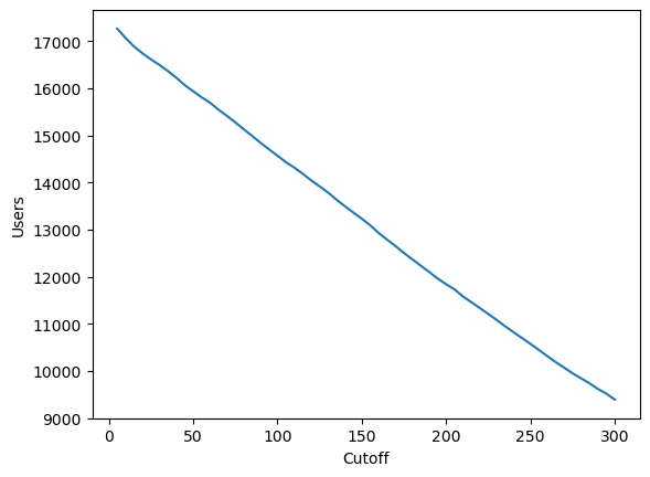
The number of users decreases linearly with increasing cutoff points (number of titles in their list). Since there is not an obvious cutoff that we can select from this, we shall arbitrarily set it to 20 interactions removing all users that have less than 20 titles in their list.
print(f'Number of unique users : {df_ratings.User_Id.nunique()}')
print(f'Number of user interactions : {df_ratings.shape[0]}')
Number of unique users : 17513
Number of user interactions : 5452192
tmp = (df_ratings.value_counts('User_Id') >= 20).reset_index()
tmp = tmp[tmp['count']==True]
df_ratings = df_ratings[df_ratings.User_Id.isin(tmp.User_Id)]
print(f'After removing users with less than 20 interactions')
print(f'Number of unique users : {df_ratings.User_Id.nunique()}')
print(f'Number of user interactions : {df_ratings.shape[0]}')
After removing users with less than 20 interactions
Number of unique users : 16744
Number of user interactions : 5445702
We see that we have 16744 users left, a decrease of aout 4.4% from the original 17513 users.
3. Baseline Model & Evaluation
As a baseline we will simply recommend users the most popular titles (based on popularity metric) that is not on their ratings list.
df_info[['MAL_Id','Name','Score','Popularity','Rank']].head()
| MAL_Id | Name | Score | Popularity | Rank | |
|---|---|---|---|---|---|
| 0 | 52991 | Sousou no Frieren | 9.276142 | 301 | 1 |
| 1 | 5114 | Fullmetal Alchemist: Brotherhood | 8.941080 | 3 | 2 |
| 2 | 9253 | Steins;Gate | 8.962588 | 13 | 3 |
| 3 | 28977 | Gintama° | 8.726812 | 341 | 4 |
| 4 | 38524 | Shingeki no Kyojin Season 3 Part 2 | 9.019487 | 21 | 5 |
def mask_user_ratings(user_ratings_df, random_state=42):
    # Sample half of rated titles as input
    input_df = user_ratings_df[user_ratings_df['Rating_Score']>0].sample(frac=0.5, random_state=random_state)
    val_df = user_ratings_df.drop(input_df.index)
    return input_df, val_df
The above function splits the user ratings dataset into an input and validation splits by sampling a user’s rated titles into the input split and placing the remaining titles into the validation split.
This approach will allow us to provide a subset of the ground truth (user’s ratings) into our recommendation system as input, and evaluate the recommendations against the remaining subset of the ground truth.
class PopularityRec:
    def __init__(self, df, anime_info_df=None):
        self.popularity = df
        self.anime_info = anime_info_df

    def predict(self, user_ratings_df, topn=10, left_on='MAL_Id', right_on='Anime_Id'):
        rec_df = self.popularity.sort_values('Popularity', ascending=True)
        rec_df = rec_df.merge(user_ratings_df, how='left', left_on=left_on, right_on=right_on)
        return rec_df.loc[rec_df[right_on].isna()][self.popularity.columns][:topn]
The above code creates a Popularity Recommendation System object that will help create predictions based on the most popular titles that the input user has not interacted with, and will be the baseline model in this notebook.
Evaluation
Two metrics will be used here
-
Mean Reciprocal Rank
\[MRR = \dfrac{1}{N}\sum_{n=1}^N \dfrac{1}{rank_i}\]
Where N is the total number of users, n is the nth user, i is the position of the first relevant item found within the recommendations
-
Normalized Discounted Cumulative Gain
\(NDCG@K = \dfrac{DCG@K}{IdealDCG@K}\) \(DCG@K = \sum_{k=1}^K \dfrac{rel_k}{log_2 (k+1)}\)
Where K is the total number of top recommendations we are evaluating, k is the kth highest predicted recommendation, rel_k is the relevance score of the recommendation at position k
IdealDCG@K is calculated by sorted the recommendations@K from order of highest relevance to lowest relevance before calculating the DGC@K. This will return the maximum achieveable DCG for the same set of ranked recommendations@K.
Essentially, the evaluation process in this notebook would be:
- - Each user will have part of their ratings list randomly sampled to use as input data
- - Recommendation system takes in input data and returns a set of ranked recommendations
- - Remaining part of the user's rating list will be used as validation data
- - MRR/NDCG will be calcualted from this validation data recommendations and the masked portion of the user's rating list
class ModelEvaluator:
    def evaluate_mrr(self, ranked_rec_df, user_input_df, user_val_df, weight=1, topn=10, left_on='MAL_Id', right_on='Anime_Id'):
        scoring_df = ranked_rec_df.merge(user_val_df, how='left', left_on=left_on, right_on=right_on)
        scoring_df = scoring_df.loc[~scoring_df[right_on].isna()][:topn]
        matched_idx = list(scoring_df[scoring_df[right_on].isin(user_val_df[right_on])].index)
        if not matched_idx:
            return 0
        return (1 * weight) / (matched_idx[0] + 1)

    def evaluate_ndcg(self, ranked_rec_df, user_input_df, user_val_df, weight=1, topn=10, left_on='MAL_Id', right_on='Anime_Id'):
        scoring_df = ranked_rec_df.merge(user_val_df, how='left', left_on=left_on, right_on=right_on)
        scoring_df = scoring_df.iloc[:topn]
        # Calculate relevance score based on how well the user interaction went
        for i in range(len(scoring_df)):
            scoring_df['rel'] = 0.0
            scoring_df.loc[scoring_df.Rating_Score == 0, 'rel'] = 0.5
            scoring_df.loc[scoring_df.Rating_Score > 0, 'rel'] = 1
            scoring_df.loc[scoring_df.Rating_Score > 5, 'rel'] = 2
            scoring_df.loc[scoring_df.Rating_Score > 8, 'rel'] = 3

        cg, icg = list(scoring_df['rel']) , sorted(scoring_df['rel'], reverse=True)
        if not cg or max(cg) == 0:
            return 0
        icg = sorted(cg, reverse=True)
        cg = list(np.array(cg) / np.array([math.log(i+1, 2) for i in range(1,len(cg) + 1)]))
        icg = list(np.array(icg) / np.array([math.log(i+1, 2) for i in range(1,len(icg) + 1)]))
        ndcg = sum(cg) / sum(icg)
        return ndcg
test_input_df, test_val_df = mask_user_ratings(df_ratings[df_ratings['User_Id']==47], random_state=1)
tester_rec = PopularityRec(df_info, df_info)
pred_df = tester_rec.predict(test_input_df, topn=10)
pred_df.head()
| MAL_Id | Name | Type | Episodes | Status | Producers | Licensors | Studios | Source | Genres | ... | Score-2 | Score-1 | Synopsis | Voice_Actors | Recommended_Ids | Recommended_Counts | Aired_Start | Aired_End | Premiered_Season | Rank | |
|---|---|---|---|---|---|---|---|---|---|---|---|---|---|---|---|---|---|---|---|---|---|
| 0 | 16498 | Shingeki no Kyojin | TV | 25.0 | Finished Airing | ['Production I.G', 'Dentsu', 'Mainichi Broadca... | ['Funimation'] | ['Wit Studio'] | Manga | ['Action', 'Award Winning', 'Drama', 'Suspense... | ... | 3828 | 9049 | Centuries ago, mankind was slaughtered to near... | ['Kaji, Yuuki', 'Ishikawa, Yui', 'Inoue, Marin... | ['28623', '37779', '26243', '20787', '5114', '... | ['111', '49', '49', '45', '44', '42', '36', '3... | 2013-04-07 | 2013-09-29 | 2.0 | 109 |
| 1 | 1535 | Death Note | TV | 37.0 | Finished Airing | ['VAP', 'Nippon Television Network', 'Shueisha... | ['VIZ Media'] | ['Madhouse'] | Manga | ['Supernatural', 'Suspense', 'Psychological', ... | ... | 3238 | 5382 | Brutal murders, petty thefts, and senseless vi... | ['Yamaguchi, Kappei', 'Miyano, Mamoru', 'Nakam... | ['1575', '19', '23283', '10620', '13601', '290... | ['633', '113', '95', '74', '67', '52', '50', '... | 2006-10-04 | 2007-06-27 | 4.0 | 79 |
| 2 | 5114 | Fullmetal Alchemist: Brotherhood | TV | 64.0 | Finished Airing | ['Aniplex', 'Square Enix', 'Mainichi Broadcast... | ['Funimation', 'Aniplex of America'] | ['Bones'] | Manga | ['Action', 'Adventure', 'Drama', 'Fantasy', 'M... | ... | 3460 | 50602 | After a horrific alchemy experiment goes wrong... | ['Park, Romi', 'Kugimiya, Rie', 'Miki, Shinich... | ['11061', '16498', '1482', '38000', '9919', '1... | ['74', '44', '21', '17', '16', '14', '14', '9'... | 2009-04-05 | 2010-07-04 | 2.0 | 2 |
| 3 | 30276 | One Punch Man | TV | 12.0 | Finished Airing | ['TV Tokyo', 'Bandai Visual', 'Lantis', 'Asats... | ['VIZ Media'] | ['Madhouse'] | Web manga | ['Action', 'Comedy', 'Adult Cast', 'Parody', '... | ... | 2027 | 3701 | The seemingly unimpressive Saitama has a rathe... | ['Furukawa, Makoto', 'Ishikawa, Kaito', 'Yuuki... | ['32182', '31964', '33255', '29803', '918', '5... | ['163', '94', '26', '21', '16', '16', '11', '1... | 2015-10-05 | 2015-12-21 | 4.0 | 129 |
| 5 | 38000 | Kimetsu no Yaiba | TV | 26.0 | Finished Airing | ['Aniplex', 'Shueisha'] | ['Aniplex of America'] | ['ufotable'] | Manga | ['Action', 'Award Winning', 'Fantasy', 'Histor... | ... | 2354 | 6186 | Ever since the death of his father, the burden... | ['Hanae, Natsuki', 'Shimono, Hiro', 'Kitou, Ak... | ['40748', '37520', '16498', '269', '5114', '31... | ['70', '42', '20', '20', '17', '15', '12', '11... | 2019-04-06 | 2019-09-28 | 2.0 | 143 |
5 rows × 40 columns
As a sanity check we have made some recommendations using User Id 47’s ratings list as shown above.
tester_eval = ModelEvaluator()
print('MRR : ', tester_eval.evaluate_mrr(pred_df, test_input_df, test_val_df, topn=10))
print('NDCG : ', tester_eval.evaluate_ndcg(pred_df, test_input_df, test_val_df, topn=10))
MRR :  0.2
NDCG :  0.430624116386567
Evaluating the predictions also reveals the above scores.
Next we shall make and evaluate recommendations for all the users in our dataset.
#calculate baseline performance
count = 0
total_mrr = 0
total_ndcg = 0
mrr_base, ndcg_base = [], []
for i in df_ratings.User_Id.unique():
    count += 1
    test_input_df, test_val_df = mask_user_ratings(df_ratings[df_ratings['User_Id']==i], random_state=1)
    pred_df = tester_rec.predict(test_input_df, topn=10)
    mrr = tester_eval.evaluate_mrr(pred_df, test_input_df, test_val_df, topn=10)
    ndcg = tester_eval.evaluate_ndcg(pred_df, test_input_df, test_val_df, topn=10)
    total_mrr += mrr
    total_ndcg += ndcg
    mrr_base.append(mrr)
    ndcg_base.append(ndcg)
def running_avg(scores):
    avgs = np.cumsum(scores)/np.array(range(1, len(scores) + 1))
    return avgs
print(f'Baseline MRR: {running_avg(mrr_base)[-1]}')
print(f'Baseline NDCG: {running_avg(ndcg_base)[-1]}')
Baseline MRR: 0.657765657823893
Baseline NDCG: 0.6612426800967172
Above we see our baseline performance that we want to beat.
4. Content Based Filtering
In this section we will explore content based filtering, where only information about the titles (i.e. descriptions, content attributes) will be used to recommend similar items to users based on their stated preferences.
As stated earlier in this notebook, we will be treating “Score” and “Popularity” features as content attributes tied to each title as they do not provide any granular user preferences information.
The underlying assumption here is that users who have interacted with certain of titles will likely enjoy other similar titles. A limitation of this is that recommendations may not be as diverse, where for example a user who has interacted with mostly Action titles will mainly be recommended similar Action titles with little deviation into other types of titles.
Titles similarities will be calculated using cosine similarity, where two similar titles should be pointing in the same direction within an inner product space.
First we will start with some data preprocessing.
df_content = df_info.copy().drop(['Aired_Start','Aired_End','Premiered_Season','Rank','Recommended_Ids','Recommended_Counts','Score-10', 'Score-9',
       'Score-8', 'Score-7', 'Score-6', 'Score-5', 'Score-4', 'Score-3',
       'Score-2', 'Score-1','Total','Watching','Completed','On-Hold','Dropped','Plan to Watch','Status','Source'], axis=1)
df_content.head()
| MAL_Id | Name | Type | Episodes | Producers | Licensors | Studios | Genres | Duration | Rating | Score | Popularity | Members | Favorites | Synopsis | Voice_Actors | |
|---|---|---|---|---|---|---|---|---|---|---|---|---|---|---|---|---|
| 0 | 52991 | Sousou no Frieren | TV | 28.0 | ['Aniplex', 'Dentsu', 'Shogakukan-Shueisha Pro... | ['None found', 'add some'] | ['Madhouse'] | ['Adventure', 'Drama', 'Fantasy', 'Shounen'] | 24 min. per ep. | PG-13 - Teens 13 or older | 9.276142 | 301 | 670859 | 35435 | During their decade-long quest to defeat the D... | ['Tanezaki, Atsumi', 'Ichinose, Kana', 'Kobaya... |
| 1 | 5114 | Fullmetal Alchemist: Brotherhood | TV | 64.0 | ['Aniplex', 'Square Enix', 'Mainichi Broadcast... | ['Funimation', 'Aniplex of America'] | ['Bones'] | ['Action', 'Adventure', 'Drama', 'Fantasy', 'M... | 24 min. per ep. | R - 17+ (violence & profanity) | 8.941080 | 3 | 3331144 | 225215 | After a horrific alchemy experiment goes wrong... | ['Park, Romi', 'Kugimiya, Rie', 'Miki, Shinich... |
| 2 | 9253 | Steins;Gate | TV | 24.0 | ['Frontier Works', 'Media Factory', 'Kadokawa ... | ['Funimation'] | ['White Fox'] | ['Drama', 'Sci-Fi', 'Suspense', 'Psychological... | 24 min. per ep. | PG-13 - Teens 13 or older | 8.962588 | 13 | 2553356 | 189031 | Eccentric scientist Rintarou Okabe has a never... | ['Miyano, Mamoru', 'Imai, Asami', 'Hanazawa, K... |
| 3 | 28977 | Gintama° | TV | 51.0 | ['TV Tokyo', 'Aniplex', 'Dentsu'] | ['Funimation', 'Crunchyroll'] | ['Bandai Namco Pictures'] | ['Action', 'Comedy', 'Sci-Fi', 'Gag Humor', 'H... | 24 min. per ep. | PG-13 - Teens 13 or older | 8.726812 | 341 | 628071 | 16610 | Gintoki, Shinpachi, and Kagura return as the f... | ['Sugita, Tomokazu', 'Kugimiya, Rie', 'Sakaguc... |
| 4 | 38524 | Shingeki no Kyojin Season 3 Part 2 | TV | 10.0 | ['Production I.G', 'Dentsu', 'Mainichi Broadca... | ['Funimation'] | ['Wit Studio'] | ['Action', 'Drama', 'Suspense', 'Gore', 'Milit... | 23 min. per ep. | R - 17+ (violence & profanity) | 9.019487 | 21 | 2262916 | 58383 | Seeking to restore humanity's diminishing hope... | ['Kamiya, Hiroshi', 'Kaji, Yuuki', 'Ishikawa, ... |
# Convert duration column to number of minutes
def convert_duration(duration):
    duration = duration.split(' ')
    duration_mins = 0
    curr_min = 1/60
    for char in duration[::-1]:
        if 'min' in char:
            curr_min = 1
        elif 'hr' in char:
            curr_min = 60
        elif char.isnumeric():
            duration_mins += int(char) * curr_min
    return duration_mins
df_content.Duration = df_content.Duration.apply(convert_duration)
df_content.Duration.head()
0    24.0
1    24.0
2    24.0
3    24.0
4    23.0
Name: Duration, dtype: float64
# Onehotencode Genre
genres = df_content['Genres'].apply(literal_eval).explode()
genres = 'genre_' + genres
genres = genres.fillna('genre_na')
df_content = df_content.drop('Genres', axis = 1).join(pd.crosstab(genres.index, genres))
df_content.head()
| MAL_Id | Name | Type | Episodes | Producers | Licensors | Studios | Duration | Rating | Score | ... | genre_Supernatural | genre_Survival | genre_Suspense | genre_Team Sports | genre_Time Travel | genre_Vampire | genre_Video Game | genre_Visual Arts | genre_Workplace | genre_na | |
|---|---|---|---|---|---|---|---|---|---|---|---|---|---|---|---|---|---|---|---|---|---|
| 0 | 52991 | Sousou no Frieren | TV | 28.0 | ['Aniplex', 'Dentsu', 'Shogakukan-Shueisha Pro... | ['None found', 'add some'] | ['Madhouse'] | 24.0 | PG-13 - Teens 13 or older | 9.276142 | ... | 0 | 0 | 0 | 0 | 0 | 0 | 0 | 0 | 0 | 0 |
| 1 | 5114 | Fullmetal Alchemist: Brotherhood | TV | 64.0 | ['Aniplex', 'Square Enix', 'Mainichi Broadcast... | ['Funimation', 'Aniplex of America'] | ['Bones'] | 24.0 | R - 17+ (violence & profanity) | 8.941080 | ... | 0 | 0 | 0 | 0 | 0 | 0 | 0 | 0 | 0 | 0 |
| 2 | 9253 | Steins;Gate | TV | 24.0 | ['Frontier Works', 'Media Factory', 'Kadokawa ... | ['Funimation'] | ['White Fox'] | 24.0 | PG-13 - Teens 13 or older | 8.962588 | ... | 0 | 0 | 1 | 0 | 1 | 0 | 0 | 0 | 0 | 0 |
| 3 | 28977 | Gintama° | TV | 51.0 | ['TV Tokyo', 'Aniplex', 'Dentsu'] | ['Funimation', 'Crunchyroll'] | ['Bandai Namco Pictures'] | 24.0 | PG-13 - Teens 13 or older | 8.726812 | ... | 0 | 0 | 0 | 0 | 0 | 0 | 0 | 0 | 0 | 0 |
| 4 | 38524 | Shingeki no Kyojin Season 3 Part 2 | TV | 10.0 | ['Production I.G', 'Dentsu', 'Mainichi Broadca... | ['Funimation'] | ['Wit Studio'] | 23.0 | R - 17+ (violence & profanity) | 9.019487 | ... | 0 | 1 | 1 | 0 | 0 | 0 | 0 | 0 | 0 | 0 |
5 rows × 90 columns
# Labelencode Type, Rating
cols = ['Type','Rating']
for col in cols:
    le = LabelEncoder()
    df_content[col] = le.fit_transform(df_content[col])
df_content[cols].head()
| Type | Rating | |
|---|---|---|
| 0 | 4 | 2 |
| 1 | 4 | 3 |
| 2 | 4 | 2 |
| 3 | 4 | 2 |
| 4 | 4 | 3 |
Above we have encoded the relevant categorical features found in the dataset, next we will need to vectorize the remaining features.
# Count Vectorize Name, Producers, Licensors, Studios, Voice_Actors,
cols = ['Name','Producers','Licensors','Studios','Voice_Actors']
sparse_total=[]
for col in cols:
    df_content[col].apply(lambda x: '' if pd.isna(x) else x.strip('[]'))
    vec = CountVectorizer()
    tmp = df_content[col]
    sparse_tmp = vec.fit_transform(tmp)
    if isinstance(sparse_total,list):
        sparse_total=sparse_tmp
    else:
        sparse_total = hstack((sparse_total, sparse_tmp))

sparse_total
<13300x18768 sparse matrix of type '<class 'numpy.int64'>'
	with 332269 stored elements in Compressed Sparse Row format>
# TFIDF Vectorize Synopsis to place emphasis on words with less occurences
sw = stopwords.words('english')
tfidf_vec = TfidfVectorizer(analyzer='word',
                            ngram_range=(1,2),
                            max_df=0.5,
                            min_df=0.001,
                            stop_words=sw)
sparse_tfidf = tfidf_vec.fit_transform(df_content['Synopsis'])
sparse_tfidf
<13300x6754 sparse matrix of type '<class 'numpy.float64'>'
	with 488956 stored elements in Compressed Sparse Row format>
For this approach we will not be combining the various arrays into a single dataframe as input. Instead we will leave them in three separate arrays
- - Dense dataframe containing numerical and categorical columns
- - Sparse array containing count vectorized features
- - Sparse array containing tfdidf vectorized synopsis
to decrease computational costs when calculating similarities between titles in the array. Recommendations made from each of the three arrays will contribute to a final list of recommendations.
df_dense = df_content.drop(['Name','Producers','Licensors','Studios','Voice_Actors','Synopsis'], axis=1)
df_dense.head()
| MAL_Id | Type | Episodes | Duration | Rating | Score | Popularity | Members | Favorites | genre_Action | ... | genre_Supernatural | genre_Survival | genre_Suspense | genre_Team Sports | genre_Time Travel | genre_Vampire | genre_Video Game | genre_Visual Arts | genre_Workplace | genre_na | |
|---|---|---|---|---|---|---|---|---|---|---|---|---|---|---|---|---|---|---|---|---|---|
| 0 | 52991 | 4 | 28.0 | 24.0 | 2 | 9.276142 | 301 | 670859 | 35435 | 0 | ... | 0 | 0 | 0 | 0 | 0 | 0 | 0 | 0 | 0 | 0 |
| 1 | 5114 | 4 | 64.0 | 24.0 | 3 | 8.941080 | 3 | 3331144 | 225215 | 1 | ... | 0 | 0 | 0 | 0 | 0 | 0 | 0 | 0 | 0 | 0 |
| 2 | 9253 | 4 | 24.0 | 24.0 | 2 | 8.962588 | 13 | 2553356 | 189031 | 0 | ... | 0 | 0 | 1 | 0 | 1 | 0 | 0 | 0 | 0 | 0 |
| 3 | 28977 | 4 | 51.0 | 24.0 | 2 | 8.726812 | 341 | 628071 | 16610 | 1 | ... | 0 | 0 | 0 | 0 | 0 | 0 | 0 | 0 | 0 | 0 |
| 4 | 38524 | 4 | 10.0 | 23.0 | 3 | 9.019487 | 21 | 2262916 | 58383 | 1 | ... | 0 | 1 | 1 | 0 | 0 | 0 | 0 | 0 | 0 | 0 |
5 rows × 84 columns
print("Missing Episodes: ", df_dense.Episodes.isna().sum())
df_dense.Episodes = df_dense.Episodes.fillna(0)
print("Missing Episodes after fillna: ", df_dense.Episodes.isna().sum())
Missing Episodes:  55
Missing Episodes after fillna:  0
scale_cols = ['Score','Members','Favorites','Episodes']
ss = StandardScaler()
df_dense[scale_cols] = ss.fit_transform(df_dense[scale_cols])
df_dense.head()
| MAL_Id | Type | Episodes | Duration | Rating | Score | Popularity | Members | Favorites | genre_Action | ... | genre_Supernatural | genre_Survival | genre_Suspense | genre_Team Sports | genre_Time Travel | genre_Vampire | genre_Video Game | genre_Visual Arts | genre_Workplace | genre_na | |
|---|---|---|---|---|---|---|---|---|---|---|---|---|---|---|---|---|---|---|---|---|---|
| 0 | 52991 | 4 | 0.271027 | 24.0 | 2 | 2.745298 | 301 | 2.705886 | 5.556849 | 0 | ... | 0 | 0 | 0 | 0 | 0 | 0 | 0 | 0 | 0 | 0 |
| 1 | 5114 | 4 | 0.952556 | 24.0 | 3 | 2.419119 | 3 | 14.743216 | 36.053453 | 1 | ... | 0 | 0 | 0 | 0 | 0 | 0 | 0 | 0 | 0 | 0 |
| 2 | 9253 | 4 | 0.195302 | 24.0 | 2 | 2.440056 | 13 | 11.223860 | 30.238883 | 0 | ... | 0 | 0 | 1 | 0 | 1 | 0 | 0 | 0 | 0 | 0 |
| 3 | 28977 | 4 | 0.706449 | 24.0 | 2 | 2.210530 | 341 | 2.512278 | 2.531775 | 1 | ... | 0 | 0 | 0 | 0 | 0 | 0 | 0 | 0 | 0 | 0 |
| 4 | 38524 | 4 | -0.069737 | 23.0 | 3 | 2.495447 | 21 | 9.909669 | 9.244467 | 1 | ... | 0 | 1 | 1 | 0 | 0 | 0 | 0 | 0 | 0 | 0 |
5 rows × 84 columns
class ContentBasedRecommender:
    def __init__(self, df_content):
        self.df_content = df_content
        self.df_dense, self.sparse_vec, self.sparse_tfidf = self.process_df(self.df_content)
        self.ref_weights = [1/math.log(len(self.df_content)-i+1, 10) + 1 for i in range(len(self.df_content))]

    def process_df(self, df_content):
        genres=df_content['Genres'].apply(literal_eval).explode()
        genres = 'genre_' + genres
        genres = genres.fillna('genre_na')
        df_content = df_content.drop('Genres', axis=1).join(pd.crosstab(genres.index, genres))

        #labelencode
        for col in ['Type','Rating']:
            le=LabelEncoder()
            df_content[col] = le.fit_transform(df_content[col])
        #Vectorize
        sparse_vec=[]
        for col in ['Name','Producers','Licensors','Studios','Voice_Actors']:
            df_content[col].apply(lambda x: '' if pd.isna(x) else x.strip('[]'))
            vec = CountVectorizer()
            tmp = df_content[col]
            sparse_tmp = vec.fit_transform(tmp)
            if isinstance(sparse_vec,list):
                sparse_vec = sparse_tmp
            else:
                sparse_vec = hstack((sparse_vec, sparse_tmp))

        tfidf_vec = TfidfVectorizer(analyzer='word',
                            ngram_range=(1,2),
                            max_df=0.5,
                            min_df=0.001,
                            stop_words=sw)
        sparse_tfidf = tfidf_vec.fit_transform(df_content['Synopsis'])

        df_dense = df_content.drop(['Name','Producers','Licensors','Studios','Voice_Actors','Synopsis'], axis=1)
        df_dense.Episodes = df_dense.Episodes.fillna(0)
        scale_cols = ['Score','Members','Favorites','Episodes']
        ss = StandardScaler()
        df_dense[scale_cols] = ss.fit_transform(df_dense[scale_cols])

        return df_dense, sparse_vec, sparse_tfidf

        self.df_dense = df_dense
        self.sparse_vec = sparse_vec
        self.sparse_tfidf = sparse_tfidf

    def get_entry(self, MAL_Id):
        title_dense = self.df_dense[self.df_dense['MAL_Id'] == MAL_Id]
        idx = title_dense.index[0]
        title_vec = self.sparse_vec[idx]
        title_tfidf = self.sparse_tfidf[idx]
        return title_dense, title_vec, title_tfidf

    def calc_sim(self, MAL_Id):
        try:
            title_dense, title_vec, title_tfidf = self.get_entry(MAL_Id)
        except:
            return None
        sim_dense = cosine_similarity(title_dense, self.df_dense)
        sim_vec = cosine_similarity(title_vec, self.sparse_vec)
        sim_tfidf = cosine_similarity(title_tfidf, self.sparse_tfidf)
        total = (sim_dense + sim_vec + sim_tfidf).argsort().flatten()
        return total


    def predict_weights(self, user_list):
        weights_df = pd.DataFrame({'Preds': self.df_content.MAL_Id, 'Weights':0})
        for MAL_Id in user_list:
            recs = self.calc_sim(MAL_Id)
            if recs is None:
                continue
            idx_recs = list(recs)
            weights_zip = list(zip(idx_recs, self.ref_weights))
            weights_zip = sorted(weights_zip)
            weights_zip = list(zip(*weights_zip))
            weights_df['Weights'] += weights_zip[1]
        weights_df['Weights'] = (weights_df['Weights'] - weights_df['Weights'].min()) / (weights_df['Weights'].max() - weights_df['Weights'].min())
        return weights_df

    def par_weights(self, user_list):
        weights_df = pd.DataFrame({'Preds': self.df_content.MAL_Id, 'Weights':0})
        recs_list=[]
        with Pool() as pool:
            for recs in pool.imap(self.calc_sim, user_list):
                if recs is None:
                    continue
                recs_list.append(recs)
        for recs in recs_list:
            idx_recs = list(recs)
            weights_zip = list(zip(idx_recs, self.ref_weights))
            weights_zip = sorted(weights_zip)
            weights_zip = list(zip(*weights_zip))
            weights_df['Weights'] += weights_zip[1]
        weights_df['Weights'] = (weights_df['Weights'] - weights_df['Weights'].min()) / (weights_df['Weights'].max() - weights_df['Weights'].min())
        return weights_df

    def par_predict(self, user_df, topn=10):
        user_list = list(user_df['Anime_Id'])
        weights_df = self.par_weights(user_list)
        res = weights_df.merge(self.df_content, how='left', left_on='Preds', right_on='MAL_Id')
        res = res.sort_values('Weights', ascending=False).loc[~res['MAL_Id'].isin(user_list)][:topn]
        return res

    def predict(self, user_df, topn=10):
        user_list = list(user_df['Anime_Id'])
        weights_df = self.predict_weights(user_list)
        res = weights_df.merge(self.df_content, how='left', left_on='Preds', right_on='MAL_Id')
        res = res.sort_values('Weights', ascending=False).loc[~res['MAL_Id'].isin(user_list)][:topn]
        return res
The above code creates a Content Based Recommendation System object that will be able to process input datasets and make recommendations. During experimentation, calculation of cosine similarity was expensive and taking too long, hence within the class I have written functions that will do the calculations in parallel to speed things up.
df_content = df_info.copy().drop(['Aired_Start','Aired_End','Premiered_Season','Rank','Recommended_Ids','Recommended_Counts','Score-10', 'Score-9',
       'Score-8', 'Score-7', 'Score-6', 'Score-5', 'Score-4', 'Score-3',
       'Score-2', 'Score-1','Total','Watching','Completed','On-Hold','Dropped','Plan to Watch','Status','Source'], axis=1)
df_content.Duration = df_content.Duration.apply(convert_duration)
df_content.Duration.head()
df_content.head()
| MAL_Id | Name | Type | Episodes | Producers | Licensors | Studios | Genres | Duration | Rating | Score | Popularity | Members | Favorites | Synopsis | Voice_Actors | |
|---|---|---|---|---|---|---|---|---|---|---|---|---|---|---|---|---|
| 0 | 52991 | Sousou no Frieren | TV | 28.0 | ['Aniplex', 'Dentsu', 'Shogakukan-Shueisha Pro... | ['None found', 'add some'] | ['Madhouse'] | ['Adventure', 'Drama', 'Fantasy', 'Shounen'] | 24.0 | PG-13 - Teens 13 or older | 9.276142 | 301 | 670859 | 35435 | During their decade-long quest to defeat the D... | ['Tanezaki, Atsumi', 'Ichinose, Kana', 'Kobaya... |
| 1 | 5114 | Fullmetal Alchemist: Brotherhood | TV | 64.0 | ['Aniplex', 'Square Enix', 'Mainichi Broadcast... | ['Funimation', 'Aniplex of America'] | ['Bones'] | ['Action', 'Adventure', 'Drama', 'Fantasy', 'M... | 24.0 | R - 17+ (violence & profanity) | 8.941080 | 3 | 3331144 | 225215 | After a horrific alchemy experiment goes wrong... | ['Park, Romi', 'Kugimiya, Rie', 'Miki, Shinich... |
| 2 | 9253 | Steins;Gate | TV | 24.0 | ['Frontier Works', 'Media Factory', 'Kadokawa ... | ['Funimation'] | ['White Fox'] | ['Drama', 'Sci-Fi', 'Suspense', 'Psychological... | 24.0 | PG-13 - Teens 13 or older | 8.962588 | 13 | 2553356 | 189031 | Eccentric scientist Rintarou Okabe has a never... | ['Miyano, Mamoru', 'Imai, Asami', 'Hanazawa, K... |
| 3 | 28977 | Gintama° | TV | 51.0 | ['TV Tokyo', 'Aniplex', 'Dentsu'] | ['Funimation', 'Crunchyroll'] | ['Bandai Namco Pictures'] | ['Action', 'Comedy', 'Sci-Fi', 'Gag Humor', 'H... | 24.0 | PG-13 - Teens 13 or older | 8.726812 | 341 | 628071 | 16610 | Gintoki, Shinpachi, and Kagura return as the f... | ['Sugita, Tomokazu', 'Kugimiya, Rie', 'Sakaguc... |
| 4 | 38524 | Shingeki no Kyojin Season 3 Part 2 | TV | 10.0 | ['Production I.G', 'Dentsu', 'Mainichi Broadca... | ['Funimation'] | ['Wit Studio'] | ['Action', 'Drama', 'Suspense', 'Gore', 'Milit... | 23.0 | R - 17+ (violence & profanity) | 9.019487 | 21 | 2262916 | 58383 | Seeking to restore humanity's diminishing hope... | ['Kamiya, Hiroshi', 'Kaji, Yuuki', 'Ishikawa, ... |
# Initialise our content based recommender object and evaluator object
content_rec = ContentBasedRecommender(df_content)
tester_eval = ModelEvaluator()
# No multiprocessing
s = datetime.now()
test_input_df, test_val_df = mask_user_ratings(df_ratings[df_ratings['User_Id']==47], random_state=1)
pred_df = content_rec.predict(test_input_df, 10)
print("Final MRR: " , tester_eval.evaluate_mrr(pred_df, test_input_df, test_val_df, topn=10))
print("Final NDCG: " , tester_eval.evaluate_ndcg(pred_df, test_input_df, test_val_df, topn=10))
print(datetime.now()-s)
Final MRR:  1.0
Final NDCG:  0.8332242176357783
0:00:01.134000
pred_df.head()
| Preds | Weights | MAL_Id | Name | Type | Episodes | Producers | Licensors | Studios | Genres | Duration | Rating | Score | Popularity | Members | Favorites | Synopsis | Voice_Actors | |
|---|---|---|---|---|---|---|---|---|---|---|---|---|---|---|---|---|---|---|
| 117 | 38474 | 0.771254 | 38474 | Yuru Camp△ Season 2 | TV | 13.0 | ['Half H.P Studio', 'MAGES.', 'DeNA'] | ['None found', 'add some'] | ['C-Station'] | ['Slice of Life', 'CGDCT', 'Iyashikei'] | 23.0 | PG-13 - Teens 13 or older | 8.504338 | 1079 | 222123 | 3039 | Having spent Christmas camping with her new fr... | ['Touyama, Nao', 'Hanamori, Yumiri', 'Toyosaki... |
| 1593 | 54005 | 0.706282 | 54005 | COLORs | ONA | 1.0 | ['TOHO animation'] | ['None found', 'add some'] | ['Wit Studio'] | ['Drama', 'Crossdressing'] | 3.0 | PG-13 - Teens 13 or older | 7.616992 | 7294 | 7142 | 50 | A girl finds herself mesmerized by a young wom... | [] |
| 1651 | 37341 | 0.691259 | 37341 | Yuru Camp△ Specials | Special | 3.0 | ['None found', 'add some'] | ['None found', 'add some'] | ['C-Station'] | ['Slice of Life', 'CGDCT', 'Iyashikei'] | 8.0 | PG-13 - Teens 13 or older | 7.581927 | 2934 | 55632 | 90 | When Chiaki Oogaki and Aoi Inuyama start the O... | ['Touyama, Nao', 'Hanamori, Yumiri', 'Toyosaki... |
| 1904 | 51958 | 0.637903 | 51958 | Kono Subarashii Sekai ni Bakuen wo! | TV | 12.0 | ['Half H.P Studio', 'Nippon Columbia', 'Atelie... | ['None found', 'add some'] | ['Drive'] | ['Comedy', 'Fantasy'] | 23.0 | PG-13 - Teens 13 or older | 7.461288 | 768 | 309112 | 1725 | Megumin is a young and passionate wizard from ... | ['Takahashi, Rie', 'Toyosaki, Aki', 'Fukushima... |
| 316 | 53888 | 0.580874 | 53888 | Spy x Family Movie: Code: White | Movie | 1.0 | ['TOHO animation', 'Shueisha'] | ['None found', 'add some'] | ['Wit Studio', 'CloverWorks'] | ['Action', 'Comedy', 'Childcare', 'Shounen'] | 110.0 | PG-13 - Teens 13 or older | 8.358056 | 2046 | 101970 | 335 | After receiving an order to be replaced in Ope... | ['Tanezaki, Atsumi', 'Hayami, Saori', 'Eguchi,... |
# Multiprocessing
s = datetime.now()
test_input_df, test_val_df = mask_user_ratings(df_ratings[df_ratings['User_Id']==47], random_state=1)
pred_df = content_rec.par_predict(test_input_df, 10)
print("Final MRR: " , tester_eval.evaluate_mrr(pred_df, test_input_df, test_val_df, topn=10))
print("Final NDCG: " , tester_eval.evaluate_ndcg(pred_df, test_input_df, test_val_df, topn=10))
print(datetime.now()-s)
Final MRR:  1.0
Final NDCG:  0.8332242176357783
0:00:00.720000
pred_df.head()
| Preds | Weights | MAL_Id | Name | Type | Episodes | Producers | Licensors | Studios | Genres | Duration | Rating | Score | Popularity | Members | Favorites | Synopsis | Voice_Actors | |
|---|---|---|---|---|---|---|---|---|---|---|---|---|---|---|---|---|---|---|
| 117 | 38474 | 0.771254 | 38474 | Yuru Camp△ Season 2 | TV | 13.0 | ['Half H.P Studio', 'MAGES.', 'DeNA'] | ['None found', 'add some'] | ['C-Station'] | ['Slice of Life', 'CGDCT', 'Iyashikei'] | 23.0 | PG-13 - Teens 13 or older | 8.504338 | 1079 | 222123 | 3039 | Having spent Christmas camping with her new fr... | ['Touyama, Nao', 'Hanamori, Yumiri', 'Toyosaki... |
| 1593 | 54005 | 0.706282 | 54005 | COLORs | ONA | 1.0 | ['TOHO animation'] | ['None found', 'add some'] | ['Wit Studio'] | ['Drama', 'Crossdressing'] | 3.0 | PG-13 - Teens 13 or older | 7.616992 | 7294 | 7142 | 50 | A girl finds herself mesmerized by a young wom... | [] |
| 1651 | 37341 | 0.691259 | 37341 | Yuru Camp△ Specials | Special | 3.0 | ['None found', 'add some'] | ['None found', 'add some'] | ['C-Station'] | ['Slice of Life', 'CGDCT', 'Iyashikei'] | 8.0 | PG-13 - Teens 13 or older | 7.581927 | 2934 | 55632 | 90 | When Chiaki Oogaki and Aoi Inuyama start the O... | ['Touyama, Nao', 'Hanamori, Yumiri', 'Toyosaki... |
| 1904 | 51958 | 0.637903 | 51958 | Kono Subarashii Sekai ni Bakuen wo! | TV | 12.0 | ['Half H.P Studio', 'Nippon Columbia', 'Atelie... | ['None found', 'add some'] | ['Drive'] | ['Comedy', 'Fantasy'] | 23.0 | PG-13 - Teens 13 or older | 7.461288 | 768 | 309112 | 1725 | Megumin is a young and passionate wizard from ... | ['Takahashi, Rie', 'Toyosaki, Aki', 'Fukushima... |
| 316 | 53888 | 0.580874 | 53888 | Spy x Family Movie: Code: White | Movie | 1.0 | ['TOHO animation', 'Shueisha'] | ['None found', 'add some'] | ['Wit Studio', 'CloverWorks'] | ['Action', 'Comedy', 'Childcare', 'Shounen'] | 110.0 | PG-13 - Teens 13 or older | 8.358056 | 2046 | 101970 | 335 | After receiving an order to be replaced in Ope... | ['Tanezaki, Atsumi', 'Hayami, Saori', 'Eguchi,... |
Sanity check on the same User Id 47 above shows that both calculations from parallel/non-parallel processing functions are the same, and the parallel calculations results in about 50% less computation time.
count, total_mrr, total_ndcg = 0, 0, 0
s = datetime.now()
number_of_samples = 1000
mrr_content, ndcg_content= [], []
for i in np.random.choice(df_ratings.User_Id.unique(), number_of_samples, replace=False):
    s_inner = datetime.now()
    count += 1
    test_input_df, test_val_df = mask_user_ratings(df_ratings[df_ratings['User_Id']==i], random_state=1)
    pred_df = content_rec.par_predict(test_input_df, 10)
    mrr =  tester_eval.evaluate_mrr(pred_df, test_input_df, test_val_df, topn=10)
    ndcg = tester_eval.evaluate_ndcg(pred_df, test_input_df, test_val_df, topn=10)
    total_mrr += mrr
    total_ndcg += ndcg
    mrr_content.append(mrr)
    ndcg_content.append(ndcg)
As the computational time required is significant higher when compared to our base model, we will evaluate our subsequent models on a subset of 380 out of the 16744 users we have in our dataset to obtain results with 95% confidence interval at 5% margin of error.
print(f'Content MRR: {running_avg(mrr_content)[-1]}')
print(f'Content NDCG: {running_avg(ndcg_content)[-1]}')
Content MRR: 0.6794964285714287
Content NDCG: 0.6826560139876724
We see that our content based recommendation system barely beats our baseline model.
5. Collaborative Filtering
Within this section we will utilise preferences and ratings information from many users to create predictions on what other similar users may be interested in.
The underlying assaumption here is that users with similar preferences and opinions would prefer the same titles as one another.
To make recommendations, the user’s input data will be appended to our ratings data and singular value decomposition (SVD) will be applied to factorize the matrix. Thereafter a dot product of the feature vector corresponding to the input user with the feature vectors corresponding to the titles will return similarity measures that we can use to make recommendations.
The same process can be applied to inputs with multiple users, this can be useful for making recommendations to groups of people looking for new titles to watch together.
df_ratings.head()
| Username | User_Id | Anime_Id | Anime_Title | Rating_Status | Rating_Score | Num_Epi_Watched | Is_Rewatching | Updated | Start_Date | |
|---|---|---|---|---|---|---|---|---|---|---|
| 0 | flerbz | 0 | 30654 | Ansatsu Kyoushitsu 2nd Season | watching | 0 | 24 | False | 2022-02-26 22:15:01+00:00 | 2022-01-29 |
| 1 | flerbz | 0 | 22789 | Barakamon | dropped | 0 | 2 | False | 2023-01-28 19:03:33+00:00 | 2022-04-06 |
| 2 | flerbz | 0 | 31964 | Boku no Hero Academia | completed | 0 | 13 | False | 2024-03-31 02:10:32+00:00 | 2024-03-30 |
| 3 | flerbz | 0 | 33486 | Boku no Hero Academia 2nd Season | completed | 0 | 25 | False | 2024-03-31 22:32:02+00:00 | 2024-03-30 |
| 4 | flerbz | 0 | 36456 | Boku no Hero Academia 3rd Season | watching | 0 | 24 | False | 2024-04-03 02:08:56+00:00 | 2024-03-31 |
def pivot_ratings(df):
    df['Mean_Score'] = 0
    mean_df = df[df['Rating_Score']>0].groupby("User_Id")['Rating_Score'].mean().reset_index().rename(columns={'Rating_Score':'mean_score'})
    df = df.merge(mean_df)
    df['Interactions'] = 0.0
    df.loc[df.Rating_Score == 0, 'Interactions'] = 2
    df.loc[df.Rating_Score-df.Mean_Score < 0, 'Interactions'] = 1
    df.loc[df.Rating_Score-df.Mean_Score == 0, 'Interactions'] = 3
    df.loc[df.Rating_Score-df.Mean_Score > 0, 'Interactions'] = 4
    df = df.pivot(index='User_Id', columns='Anime_Id', values='Interactions').fillna(0)
    return df
The above function calculates the mean ratings per rated title for each user, and subtracts this mean from all of the ratings the user has made to remove rating biases. An interaction score is then computed based on how well the user rated the interaction. A pivot is then applied to the dataframe preparing it for modeling.
df_cf = df_ratings.copy()
df_cf = pivot_ratings(df_cf)
df_cf.head()
| Anime_Id | 1 | 5 | 6 | 7 | 8 | 15 | 16 | 17 | 18 | 19 | ... | 58564 | 58567 | 58569 | 58572 | 58573 | 58592 | 58600 | 58603 | 58614 | 58632 |
|---|---|---|---|---|---|---|---|---|---|---|---|---|---|---|---|---|---|---|---|---|---|
| User_Id | |||||||||||||||||||||
| 0 | 0.0 | 0.0 | 0.0 | 0.0 | 0.0 | 0.0 | 0.0 | 0.0 | 0.0 | 0.0 | ... | 0.0 | 0.0 | 0.0 | 0.0 | 0.0 | 0.0 | 0.0 | 0.0 | 0.0 | 0.0 |
| 1 | 3.0 | 0.0 | 3.0 | 0.0 | 0.0 | 0.0 | 0.0 | 0.0 | 0.0 | 3.0 | ... | 0.0 | 0.0 | 0.0 | 3.0 | 0.0 | 0.0 | 0.0 | 0.0 | 0.0 | 0.0 |
| 2 | 0.0 | 0.0 | 0.0 | 0.0 | 0.0 | 0.0 | 0.0 | 0.0 | 0.0 | 0.0 | ... | 0.0 | 0.0 | 0.0 | 0.0 | 0.0 | 0.0 | 0.0 | 0.0 | 0.0 | 0.0 |
| 4 | 0.0 | 0.0 | 0.0 | 0.0 | 0.0 | 0.0 | 0.0 | 0.0 | 0.0 | 4.0 | ... | 0.0 | 0.0 | 0.0 | 0.0 | 0.0 | 0.0 | 0.0 | 0.0 | 0.0 | 0.0 |
| 5 | 0.0 | 0.0 | 0.0 | 0.0 | 0.0 | 0.0 | 0.0 | 0.0 | 0.0 | 0.0 | ... | 0.0 | 0.0 | 0.0 | 0.0 | 0.0 | 0.0 | 0.0 | 0.0 | 0.0 | 0.0 |
5 rows × 17178 columns
df_cf.shape
(15615, 17178)
test_input_df_original, test_val_df = mask_user_ratings(df_ratings[df_ratings['User_Id']==47], random_state=1)
test_input_df = pivot_ratings(test_input_df_original)
test_input_df
| Anime_Id | 1 | 5 | 32 | 4037 | 11757 | 14719 | 30831 | 31933 | 34798 | 38040 | ... | 49026 | 50265 | 50602 | 50710 | 51179 | 52701 | 52741 | 53887 | 54829 | 55818 |
|---|---|---|---|---|---|---|---|---|---|---|---|---|---|---|---|---|---|---|---|---|---|
| User_Id | |||||||||||||||||||||
| 47 | 4.0 | 4.0 | 4.0 | 4.0 | 4.0 | 4.0 | 4.0 | 4.0 | 4.0 | 4.0 | ... | 4.0 | 4.0 | 4.0 | 4.0 | 4.0 | 4.0 | 4.0 | 4.0 | 4.0 | 4.0 |
1 rows × 21 columns
# calculating new index labels for the test input
new_index = pd.Series(list(range(df_cf.index[-1] + 1, df_cf.index[-1] + 1 + len(test_input_df))))
new_index
0    20011
dtype: int64
# Ratings dataset + user input data
df_cf = pd.concat([df_cf, test_input_df.set_index(new_index)]).fillna(0)
df_cf
| Anime_Id | 1 | 5 | 6 | 7 | 8 | 15 | 16 | 17 | 18 | 19 | ... | 58564 | 58567 | 58569 | 58572 | 58573 | 58592 | 58600 | 58603 | 58614 | 58632 |
|---|---|---|---|---|---|---|---|---|---|---|---|---|---|---|---|---|---|---|---|---|---|
| 0 | 0.0 | 0.0 | 0.0 | 0.0 | 0.0 | 0.0 | 0.0 | 0.0 | 0.0 | 0.0 | ... | 0.0 | 0.0 | 0.0 | 0.0 | 0.0 | 0.0 | 0.0 | 0.0 | 0.0 | 0.0 |
| 1 | 3.0 | 0.0 | 3.0 | 0.0 | 0.0 | 0.0 | 0.0 | 0.0 | 0.0 | 3.0 | ... | 0.0 | 0.0 | 0.0 | 3.0 | 0.0 | 0.0 | 0.0 | 0.0 | 0.0 | 0.0 |
| 2 | 0.0 | 0.0 | 0.0 | 0.0 | 0.0 | 0.0 | 0.0 | 0.0 | 0.0 | 0.0 | ... | 0.0 | 0.0 | 0.0 | 0.0 | 0.0 | 0.0 | 0.0 | 0.0 | 0.0 | 0.0 |
| 4 | 0.0 | 0.0 | 0.0 | 0.0 | 0.0 | 0.0 | 0.0 | 0.0 | 0.0 | 4.0 | ... | 0.0 | 0.0 | 0.0 | 0.0 | 0.0 | 0.0 | 0.0 | 0.0 | 0.0 | 0.0 |
| 5 | 0.0 | 0.0 | 0.0 | 0.0 | 0.0 | 0.0 | 0.0 | 0.0 | 0.0 | 0.0 | ... | 0.0 | 0.0 | 0.0 | 0.0 | 0.0 | 0.0 | 0.0 | 0.0 | 0.0 | 0.0 |
| ... | ... | ... | ... | ... | ... | ... | ... | ... | ... | ... | ... | ... | ... | ... | ... | ... | ... | ... | ... | ... | ... |
| 20007 | 4.0 | 0.0 | 3.0 | 0.0 | 0.0 | 0.0 | 0.0 | 0.0 | 4.0 | 0.0 | ... | 0.0 | 0.0 | 0.0 | 0.0 | 0.0 | 0.0 | 0.0 | 0.0 | 0.0 | 0.0 |
| 20008 | 0.0 | 0.0 | 0.0 | 0.0 | 0.0 | 3.0 | 0.0 | 0.0 | 0.0 | 4.0 | ... | 0.0 | 0.0 | 0.0 | 0.0 | 0.0 | 0.0 | 0.0 | 0.0 | 0.0 | 0.0 |
| 20009 | 4.0 | 0.0 | 3.0 | 0.0 | 0.0 | 0.0 | 0.0 | 0.0 | 0.0 | 3.0 | ... | 0.0 | 0.0 | 0.0 | 0.0 | 0.0 | 0.0 | 0.0 | 0.0 | 0.0 | 0.0 |
| 20010 | 4.0 | 4.0 | 4.0 | 0.0 | 0.0 | 0.0 | 0.0 | 0.0 | 0.0 | 4.0 | ... | 0.0 | 0.0 | 0.0 | 0.0 | 0.0 | 0.0 | 0.0 | 0.0 | 0.0 | 0.0 |
| 20011 | 4.0 | 4.0 | 0.0 | 0.0 | 0.0 | 0.0 | 0.0 | 0.0 | 0.0 | 0.0 | ... | 0.0 | 0.0 | 0.0 | 0.0 | 0.0 | 0.0 | 0.0 | 0.0 | 0.0 | 0.0 |
15616 rows × 17178 columns
# Applying SVD on sparse matrix
s = datetime.now()
sparse_cf = csr_matrix(df_cf)
U, sigma, Vt = svds(sparse_cf)
print(datetime.now() - s)
0:00:04.596998
U.shape
(15616, 6)
Vt.shape
(6, 17178)
sigma = np.diag(sigma)
# Reconstruct matrix and normalizing the measures
all_ratings = np.dot(np.dot(U, sigma), Vt)
all_ratings = (all_ratings - all_ratings.min()) / (all_ratings.max() - all_ratings.min())
all_ratings.shape
(15616, 17178)
# Show our reconstructed matrix, for each row of user_id the columns show how closely aligned they are with each anime title
df_cf_pred = pd.DataFrame(all_ratings, columns = df_cf.columns, index = df_cf.index)
df_cf_pred
| Anime_Id | 1 | 5 | 6 | 7 | 8 | 15 | 16 | 17 | 18 | 19 | ... | 58564 | 58567 | 58569 | 58572 | 58573 | 58592 | 58600 | 58603 | 58614 | 58632 |
|---|---|---|---|---|---|---|---|---|---|---|---|---|---|---|---|---|---|---|---|---|---|
| 0 | 0.322143 | 0.281029 | 0.284811 | 0.265056 | 0.264715 | 0.270996 | 0.261508 | 0.264742 | 0.271192 | 0.309478 | ... | 0.264124 | 0.276174 | 0.264103 | 0.270113 | 0.268170 | 0.265395 | 0.264182 | 0.264130 | 0.264266 | 0.264123 |
| 1 | 0.426405 | 0.302308 | 0.289836 | 0.264833 | 0.262356 | 0.255552 | 0.300901 | 0.262838 | 0.282760 | 0.416440 | ... | 0.264126 | 0.313230 | 0.264115 | 0.285468 | 0.267381 | 0.268286 | 0.267278 | 0.264312 | 0.264614 | 0.264151 |
| 2 | 0.355228 | 0.353592 | 0.215732 | 0.261275 | 0.276188 | 0.306569 | 0.335670 | 0.266856 | 0.261291 | 0.128861 | ... | 0.264151 | 0.243649 | 0.264216 | 0.253360 | 0.270926 | 0.263537 | 0.269985 | 0.265600 | 0.264068 | 0.264374 |
| 4 | 0.335182 | 0.252427 | 0.282612 | 0.265102 | 0.265241 | 0.278636 | 0.267611 | 0.264956 | 0.287778 | 0.306845 | ... | 0.264129 | 0.291591 | 0.264180 | 0.277689 | 0.264350 | 0.267018 | 0.264216 | 0.264182 | 0.264060 | 0.264139 |
| 5 | 0.196523 | 0.209384 | 0.235906 | 0.261257 | 0.262673 | 0.249039 | 0.244840 | 0.261336 | 0.264960 | 0.233427 | ... | 0.264131 | 0.296764 | 0.264170 | 0.282507 | 0.261342 | 0.268099 | 0.265622 | 0.264338 | 0.264221 | 0.264163 |
| ... | ... | ... | ... | ... | ... | ... | ... | ... | ... | ... | ... | ... | ... | ... | ... | ... | ... | ... | ... | ... | ... |
| 20007 | 0.489428 | 0.306336 | 0.338105 | 0.269412 | 0.263843 | 0.272239 | 0.307359 | 0.264999 | 0.296388 | 0.462530 | ... | 0.264125 | 0.293219 | 0.264164 | 0.272673 | 0.261987 | 0.265958 | 0.264268 | 0.264092 | 0.264209 | 0.264122 |
| 20008 | 0.543922 | 0.333727 | 0.363319 | 0.268517 | 0.266733 | 0.287688 | 0.256264 | 0.265529 | 0.297220 | 0.494144 | ... | 0.264127 | 0.331264 | 0.264056 | 0.296463 | 0.279677 | 0.271361 | 0.265253 | 0.264365 | 0.264831 | 0.264159 |
| 20009 | 0.485117 | 0.329416 | 0.334906 | 0.268958 | 0.264527 | 0.280297 | 0.299506 | 0.266346 | 0.291095 | 0.443311 | ... | 0.264120 | 0.283117 | 0.264103 | 0.269180 | 0.268408 | 0.264956 | 0.263968 | 0.263980 | 0.264310 | 0.264098 |
| 20010 | 0.602587 | 0.379842 | 0.355045 | 0.271216 | 0.264315 | 0.282937 | 0.351978 | 0.267386 | 0.300561 | 0.525480 | ... | 0.264118 | 0.276331 | 0.264112 | 0.261242 | 0.266583 | 0.263021 | 0.264786 | 0.263954 | 0.264307 | 0.264092 |
| 20011 | 0.281417 | 0.267700 | 0.271291 | 0.264485 | 0.263932 | 0.262970 | 0.264506 | 0.263964 | 0.265495 | 0.284469 | ... | 0.264124 | 0.268596 | 0.264120 | 0.266007 | 0.264448 | 0.264542 | 0.264210 | 0.264130 | 0.264178 | 0.264125 |
15616 rows × 17178 columns
test_pred = df_cf_pred.loc[20011].sort_values(ascending=False).reset_index()
test_pred = test_pred.loc[~test_pred['Anime_Id'].isin(test_input_df_original['Anime_Id'])]
test_pred.head()
| Anime_Id | 20011 | |
|---|---|---|
| 1 | 16498 | 0.308918 |
| 2 | 25777 | 0.306242 |
| 3 | 35760 | 0.306020 |
| 4 | 38524 | 0.305755 |
| 5 | 40028 | 0.305438 |
tester_eval = ModelEvaluator()
print('MRR : ', tester_eval.evaluate_mrr(test_pred, None, test_val_df, topn=10, left_on='Anime_Id'))
print('NDCG : ', tester_eval.evaluate_ndcg(test_pred, None, test_val_df, topn=10, left_on='Anime_Id'))
MRR :  0.14285714285714285
NDCG :  0.32166167872792356
# User only interacted with 1 title out of the top 10 predictions
test_pred.iloc[:10].merge(test_val_df, how='left')
| Anime_Id | 20011 | Username | User_Id | Anime_Title | Rating_Status | Rating_Score | Num_Epi_Watched | Is_Rewatching | Updated | Start_Date | |
|---|---|---|---|---|---|---|---|---|---|---|---|
| 0 | 16498 | 0.308918 | NaN | NaN | NaN | NaN | NaN | NaN | NaN | NaN | NaN |
| 1 | 25777 | 0.306242 | NaN | NaN | NaN | NaN | NaN | NaN | NaN | NaN | NaN |
| 2 | 35760 | 0.306020 | NaN | NaN | NaN | NaN | NaN | NaN | NaN | NaN | NaN |
| 3 | 38524 | 0.305755 | NaN | NaN | NaN | NaN | NaN | NaN | NaN | NaN | NaN |
| 4 | 40028 | 0.305438 | NaN | NaN | NaN | NaN | NaN | NaN | NaN | NaN | NaN |
| 5 | 40748 | 0.304172 | NaN | NaN | NaN | NaN | NaN | NaN | NaN | NaN | NaN |
| 6 | 38000 | 0.304036 | Pynkmouth | 47.0 | Kimetsu no Yaiba | plan_to_watch | 0.0 | 0.0 | False | 2021-03-18 22:08:00+00:00 | NaN |
| 7 | 48583 | 0.302796 | NaN | NaN | NaN | NaN | NaN | NaN | NaN | NaN | NaN |
| 8 | 47778 | 0.301383 | NaN | NaN | NaN | NaN | NaN | NaN | NaN | NaN | NaN |
| 9 | 52991 | 0.301243 | Pynkmouth | 47.0 | Sousou no Frieren | completed | 6.0 | 28.0 | False | 2024-04-11 10:28:04+00:00 | NaN |
class CollaborativeRecommender:
    def __init__(self, df_cf):
        self.df_original = df_cf
        self.df_anime_id = df_cf.groupby(['Anime_Id','Anime_Title']).count().reset_index()[['Anime_Id','Anime_Title']]

    def process_df(self, df):
        df['Mean_Score'] = 0
        mean_df = df[df['Rating_Score']>0].groupby("User_Id")['Rating_Score'].mean().reset_index().rename(columns={'Rating_Score':'mean_score'})
        df = df.merge(mean_df)
        df['Interactions'] = 0.0
        df.loc[df.Rating_Score == 0, 'Interactions'] = 2
        df.loc[df.Rating_Score-df.Mean_Score < 0, 'Interactions'] = 1
        df.loc[df.Rating_Score-df.Mean_Score == 0, 'Interactions'] = 3
        df.loc[df.Rating_Score-df.Mean_Score > 0, 'Interactions'] = 4
        df = df.pivot(index='User_Id', columns='Anime_Id', values='Interactions').fillna(0)
        return df

    def predict_dec(self, user_df, k=15):
        max_uid = self.df_original.User_Id.max()
        for i, uid in enumerate(user_df.User_Id.unique()):
            user_df.loc[user_df.User_Id==uid, 'User_Id'] = max_uid + 1 + i
        user_df = pd.concat([self.df_original, user_df])
        user_cf = self.process_df(user_df)
        sparse_cf = csr_matrix(user_cf)
        U, sigma, Vt = svds(sparse_cf)
        return U, sigma, Vt, user_cf.columns, user_cf.index

    def predict(self, user_df, topn=10, k=15):
        # Reconstruct matrix to find similarities
        U, sigma, Vt, new_col, new_index = self.predict_dec(user_df, k)
        sigma = np.diag(sigma)
        all_ratings = np.dot(np.dot(U,sigma), Vt)
        all_ratings = (all_ratings - all_ratings.min()) / (all_ratings.max() - all_ratings.min())

        # Construct output dataframe, collecting weights from the number of user we have predicted on
        df_cf_pred = pd.DataFrame(all_ratings, columns=new_col, index=new_index)
        num_users = user_df.User_Id.nunique()
        res = df_cf_pred.iloc[-num_users:].T
        if num_users == 1:
            res = res.sort_values(res.columns[0],ascending=False).reset_index()
            res = res.loc[~res['Anime_Id'].isin(user_df['Anime_Id'])][:topn]
        else:
            res = res.reset_index()
            res = res.loc[~res['Anime_Id'].isin(user_df['Anime_Id'])]
        return res
As before, we have code to create an object for our Collaborative Recommender System, taking in some inputs and producing recommendations.
# 3 Samples, all anime titles from dataset
df_cf = df_ratings.copy()
cf_rec = CollaborativeRecommender(df_cf)
tester_eval = ModelEvaluator()

count, total_mrr, total_ndcg = 0, 0, 0
s = datetime.now()
number_of_samples = 3
print(f"Number of Anime Titles within our dataset: {df_cf.Anime_Id.nunique()}")
for i in np.random.choice(df_ratings.User_Id.unique(), number_of_samples, replace=False):
    s_inner = datetime.now()
    count += 1
    test_input_df, test_val_df = mask_user_ratings(df_ratings[df_ratings['User_Id']==i], random_state=1)
    pred_df = cf_rec.predict(test_input_df, 10)
    total_mrr += tester_eval.evaluate_mrr(pred_df, test_input_df, test_val_df, topn=10, left_on='Anime_Id')
    total_ndcg += tester_eval.evaluate_ndcg(pred_df, test_input_df, test_val_df, topn=10, left_on='Anime_Id')
    if not count % 10:
        print(f'Time Elapsed : {datetime.now()-s}')
    print(f"Loop Number {count}, User Id {i}, Time Taken {datetime.now()-s_inner}")
print("Final MRR: " , total_mrr/count)
print("Final NDCG: " , total_ndcg/count)
Number of Anime Titles within our dataset: 17365
Loop Number 1, User Id 13830, Time Taken 0:00:08.383678
Loop Number 2, User Id 4062, Time Taken 0:00:08.232498
Loop Number 3, User Id 17416, Time Taken 0:00:08.202000
Final MRR:  0.7777777777777778
Final NDCG:  0.8000865280044508
Sanity check with 3 samples looks fine, compared to previous approaches this does take a significantly longer time to compute.
df_cf = df_ratings.copy()
cf_rec = CollaborativeRecommender(df_cf)
tester_eval = ModelEvaluator()

count, total_mrr, total_ndcg = 0, 0, 0
s = datetime.now()
number_of_samples = 1000
mrr_collab, ndcg_collab = [], []
for i in np.random.choice(df_ratings.User_Id.unique(), number_of_samples, replace=False):
    s_inner = datetime.now()
    count += 1
    test_input_df, test_val_df = mask_user_ratings(df_ratings[df_ratings['User_Id']==i], random_state=1)
    pred_df = cf_rec.predict(test_input_df, 10)
    mrr = tester_eval.evaluate_mrr(pred_df, test_input_df, test_val_df, topn=10, left_on='Anime_Id')
    ndcg = tester_eval.evaluate_ndcg(pred_df, test_input_df, test_val_df, topn=10, left_on='Anime_Id')
    total_mrr += mrr
    total_ndcg += ndcg
    mrr_collab.append(mrr)
    ndcg_collab.append(ndcg)
print(f'Collab MRR: {running_avg(mrr_collab)[-1]}')
print(f'Collab NDCG: {running_avg(ndcg_collab)[-1]}')
Collab MRR: 0.8626269841269844
Collab NDCG: 0.801510934536861
The performance of the collaborative approach is significantly better than the baseline and content base recommndations, suggesting that the assumption that similar users will like similar titles may have some truth in it. A possible explanation for why the performance is not better is that our SVD is not able to accurately recreate the original matrix due to the chosen low number of singular values computed.
Below is a sanity check with 3 samples again, but with obscure titles that have less than 3 ratings removed from the computation
Surprisingly, the performance of this approach is worse than our baseline and content base recommendations. A possible explanation is that our SVD is not able to accurately recreate the original matrix due to the chosen low number of singular values computed. If this approach is re-evaluated with a higher number of singlular values with similarly poor results, it will suggest that the original assumption of similar users liking similar titles is not entire accurate.
Below is a sanity check with 3 samples again, but with obscure titles that have less than 3 ratings removed from the computation
# Remove titles with less than 10 user ratings
df_ratings_subset = df_ratings[['Anime_Id','Anime_Title']].value_counts().reset_index()
df_ratings_subset = df_ratings_subset[df_ratings_subset['count'] >= 10]
df_cf_subset = df_ratings[df_ratings.Anime_Id.isin(df_ratings_subset.Anime_Id)]
print(f"Original number of titles: {df_ratings.Anime_Title.nunique()}")
print(f"Trimmed number of titles: {df_ratings_subset.Anime_Title.nunique()}")
Original number of titles: 17364
Trimmed number of titles: 10559
# 3 Samples, trimmed anime titles from dataset
cf_rec = CollaborativeRecommender(df_cf_subset)
tester_eval = ModelEvaluator()

count, total_mrr, total_ndcg = 0, 0, 0
s = datetime.now()
number_of_samples = 3
print(f"Number of Anime Titles with >= 10 user ratings within our dataset: {df_cf_subset.Anime_Id.nunique()}")
for i in np.random.choice(df_ratings.User_Id.unique(), number_of_samples, replace=False):
    s_inner = datetime.now()
    count += 1
    test_input_df, test_val_df = mask_user_ratings(df_ratings[df_ratings['User_Id']==i], random_state=1)
    pred_df = cf_rec.predict(test_input_df, 10)
    total_mrr += tester_eval.evaluate_mrr(pred_df, test_input_df, test_val_df, topn=10, left_on='Anime_Id')
    total_ndcg += tester_eval.evaluate_ndcg(pred_df, test_input_df, test_val_df, topn=10, left_on='Anime_Id')
    if not count % 10:
        print(f'Time Elapsed : {datetime.now()-s}')
    print(f"Loop Number {count}, User Id {i}, Time Taken {datetime.now()-s_inner}")
print("Final MRR: " , total_mrr/count)
print("Final NDCG: " , total_ndcg/count)
Number of Anime Titles with >= 10 user ratings within our dataset: 10559
Loop Number 1, User Id 19564, Time Taken 0:00:06.346500
Loop Number 2, User Id 8772, Time Taken 0:00:06.117500
Loop Number 3, User Id 16816, Time Taken 0:00:06.155999
Final MRR:  0.75
Final NDCG:  0.7081818849660128
By trimming the really obscure titles from the dataset we are able to reduce computational times significantly.
6. Hybrid Recommendation
For our hybrid approach we will combine both the Content Based and Collaborative approaches we have explored.
For simplicity’s sake we will place a 0.5 weightage for each of the approaches.
Similarity measures from each of these two approaches will be computed separately and standardised so that they are comparable. The final measure will be a combination of the standardised scores based on their weightages.
class HybridRecommender:
    def __init__(self, cb_model, cf_model, df_content, df_ratings, cb_weight=0.5):
        self.cb_model = cb_model(df_content)
        self.cf_model = cf_model(df_ratings)
        self.cb_weight = cb_weight
        self.cf_weight = 1 - cb_weight
        self.n = df_ratings.Anime_Id.nunique()

    def predict(self, user_df, topn=10):
        num_users = user_df.User_Id.nunique()
        cb_pred = self.cb_model.predict(user_df, self.n)
        cf_pred = self.cf_model.predict(user_df, self.n)

        # Normalize scores from both predictions
        ss = StandardScaler()
        cb_pred['ss'] = ss.fit_transform(cb_pred['Weights'].values.reshape(-1,1))
        cf_cols = ['ss_' + str(col) for col in cf_pred.columns[-1:]]
        if num_users == 1:
            cf_pred[cf_cols] = ss.fit_transform(cf_pred[cf_pred.columns[-1]].values.reshape(-1,1))
        else:
            cf_pred[cf_cols] = ss.fit_transform(cf_pred[cf_pred.columns[1:]])

        combined_pred = cf_pred.merge(cb_pred[['ss','MAL_Id','Name','Score','Popularity']], how='left', left_on='Anime_Id', right_on='MAL_Id')
        combined_pred['Final_Score'] = self.cf_weight*combined_pred[cf_cols].sum(axis=1) + self.cb_weight*combined_pred['ss']
        combined_pred = combined_pred.sort_values('Final_Score', ascending=False)
        return combined_pred[:topn]
# Remove titles with less than 10 user ratings
df_ratings_subset = df_ratings[['Anime_Id','Anime_Title']].value_counts().reset_index()
df_ratings_subset = df_ratings_subset[df_ratings_subset['count'] >= 10]
df_cf_subset = df_ratings[df_ratings.Anime_Id.isin(df_ratings_subset.Anime_Id)]
tester_eval = ModelEvaluator()

hyb_rec = HybridRecommender(ContentBasedRecommender, CollaborativeRecommender, df_content, df_cf_subset, cb_weight = 0.5)
count, total_mrr, total_ndcg = 0, 0, 0
s = datetime.now()
number_of_samples = 1000
print(f"Number of Anime Titles with >= 10 user ratings within our dataset: {df_cf_subset.Anime_Id.nunique()}")
mrr_hybrid, ndcg_hybrid = [], []
for i in np.random.choice(df_ratings.User_Id.unique(), number_of_samples, replace=False):
    s_inner = datetime.now()
    count += 1
    test_input_df, test_val_df = mask_user_ratings(df_ratings[df_ratings['User_Id']==i], random_state=1)
    if len(test_input_df) == 0:
        continue
    pred_df = hyb_rec.predict(test_input_df, 10)
    mrr = tester_eval.evaluate_mrr(pred_df, test_input_df, test_val_df, topn=10, left_on='Anime_Id')
    ndcg = tester_eval.evaluate_ndcg(pred_df, test_input_df, test_val_df, topn=10, left_on='Anime_Id')
    total_mrr += mrr
    total_ndcg += ndcg
    mrr_hybrid.append(mrr)
    ndcg_hybrid.append(ndcg)
print(f'Hybrid MRR: {running_avg(mrr_hybrid)[-1]}')
print(f'Hybrid NDCG: {running_avg(ndcg_hybrid)[-1]}')
Hybrid MRR: 0.9044096472282224
Hybrid NDCG: 0.8450766763118507
mrr_base_trunc = mrr_base[-1000:]
ndcg_base_trunc = ndcg_base[-1000:]
res = [mrr_base_trunc, ndcg_base_trunc, mrr_content,ndcg_content,mrr_collab,ndcg_collab,mrr_hybrid,ndcg_hybrid]
res = [running_avg(scores) for scores in res]
# Extract mrr and ndcg from list of all scores
mrr_res = res[::2]
ndcg_res = res[1::2]
# Plot averaged cumulative performance over time
fig, ax = plt.subplots(2,1, figsize=(8,8))
mrr_label = ['MRR_Base','MRR_Content','MRR_Collab','MRR_Hybrid']
ndcg_label = ['NDCG_Base','NDCG_Content','NDCG_Collab','NDCG_Hybrid']
for i, r in enumerate(mrr_res):
    sns.lineplot(r, ax = ax[0], label = mrr_label[i])
for i, r in enumerate(ndcg_res):
    sns.lineplot(r, ax = ax[1], label = ndcg_label[i])
plt.xlabel("Samples")
plt.ylabel("Cumulative Average")
plt.suptitle("Cumulative Score Plot")
ax[0].title.set_text("MRR")
ax[1].title.set_text("NDCG")
plt.show()
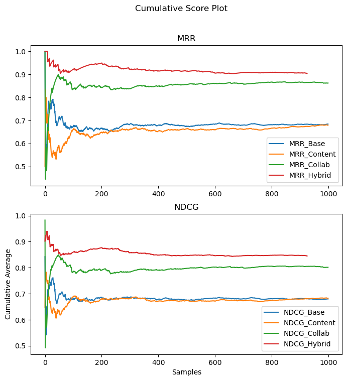
The performance of the hybrid approach appears to be significantly better than our previous two approaches and the baseline. This may be due to the limitations mentioned in our previous sections where the content based approach tend to stick to titles of the same kind, and for collaborative approach similar users tend to like similar titles, may not translate well to actual user behaviour. The higher performance of the hybrid approach suggests that in reality users may mainly enjoy titles of the same type while also seeking out some diversity in their interactions, where this diversity coincides with other similar users have interacted with.
final_res = [i[-1] for i in res]
final_mrr = final_res[::2]
final_ndcg = final_res[1::2]
final_results = pd.DataFrame({'MRR':final_mrr, "NDCG":final_ndcg}, index=['Baseline','Content','Collab','Hybrid'])
fig,ax = plt.subplots()
c_map = plt.cm.get_cmap('coolwarm').reversed()
im = ax.imshow(final_results.values, cmap=c_map)
cbar = ax.figure.colorbar(im, ax=ax)
cbar.ax.set_ylabel("Performance (Higher is better)", rotation=-90, va="bottom")

ax.set_xticks(np.arange(final_results.shape[1]), labels=final_results.columns)
ax.set_yticks(np.arange(final_results.shape[0]), labels=final_results.index)
for i in range(final_results.shape[0]):
    for j in range(final_results.shape[1]):
        text = ax.text(j, i, round(final_results.iloc[i, j], 3),
                      ha='center', va='center', color='w')
plt.tight_layout()
plt.title('Comparison of Final Performances')
Text(0.5, 1.0, 'Comparison of Final Performances')
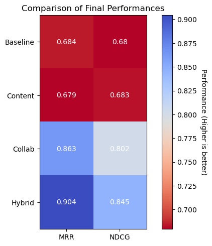
Above we see a visual representation of the scores that were seen in this notebook, with the hybrid approach coming out on top compared to our baseline and the other two approaches.
7. Conclusion
In this notebook we have explored different approaches to a recommendation system and discussed some possible limitations and their implications or solutions. For the datasets used, we have shown that the hybrid approach performed best out of the ones tested.
Further improvements can be made to our approaches, some key ones are:
- - Utilizing the review dataset to provide additional information for our titles
- - Improving computational performances of the approaches
- - Incorporating additional contextual information such as time to further improve the recommendations
- - Exploring more advanced techniques to calculate recommendations