HDB Prices from 1990 to 2024
Contents
- Introduction
- Data Cleaning/Feature Engineering
- Data Exploration
3.1 How quickly are Resale Flats prices rising?
3.2 How does flat model, storey range, and size affect prices?
3.3 How does location affect prices?
3.4 How does lease affect prices?
3.5 Are flats getting smaller?
1. Introduction
In this notebook we will explore a few HDB Resale Prices datasets from Jan1990 to Dec2014 obtained from data.gov website. The datasets are structured similarly except for the date each datapoint was sampled. Prior to Mar 2012 it’s based on approval date, beyond that it’s based on registration date.
Proper definition of these dates cannot be found, inferring from HDB’s Site I assume that the differences are as follows:
- Approval Date - Acceptance of Resale Application
- Registration Date - Unclear if this is when seller Register Intent to Sell or when Resale Application is Submitted, possible gap of ~2 weeks
For the purposes of this notebook the slight discrepancies between these two dates are not that important, hence we will be treating them the same way.
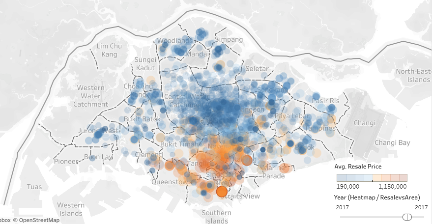
A Tableau dashboard for quick exploration and visualization of the dataset has been created. A component showing geographical resale price differences is shown in the image below
2. Data Cleaning / Feature Engineering
Since the datasets are separated into multiple .csv files, we will be loading them into memory to create a combined file containing all the data to work with.
import pandas as pd
import numpy as np
import os
import glob

import geocoder
import geopandas as gpd

import matplotlib.pyplot as plt
import matplotlib.ticker as mticker
import matplotlib.dates as md
import seaborn as sns
import ipywidgets
from ipywidgets import interact
import warnings
from scipy.optimize import curve_fit
warnings.filterwarnings('ignore')
sns.set_palette('Paired')
csvs = glob.glob('Resale*.{}'.format('csv'))
csvs
['ResaleFlatPricesBasedonApprovalDate19901999.csv',
 'ResaleFlatPricesBasedonApprovalDate2000Feb2012.csv',
 'ResaleFlatPricesBasedonRegistrationDateFromJan2015toDec2016.csv',
 'ResaleflatpricesbasedonregistrationdatefromJan2017onwards.csv',
 'ResaleFlatPricesBasedonRegistrationDateFromMar2012toDec2014.csv']
df0 = pd.read_csv(csvs[0])
df0.head()
| month | town | flat_type | block | street_name | storey_range | floor_area_sqm | flat_model | lease_commence_date | resale_price | |
|---|---|---|---|---|---|---|---|---|---|---|
| 0 | 1990-01 | ANG MO KIO | 1 ROOM | 309 | ANG MO KIO AVE 1 | 10 TO 12 | 31.0 | IMPROVED | 1977 | 9000 |
| 1 | 1990-01 | ANG MO KIO | 1 ROOM | 309 | ANG MO KIO AVE 1 | 04 TO 06 | 31.0 | IMPROVED | 1977 | 6000 |
| 2 | 1990-01 | ANG MO KIO | 1 ROOM | 309 | ANG MO KIO AVE 1 | 10 TO 12 | 31.0 | IMPROVED | 1977 | 8000 |
| 3 | 1990-01 | ANG MO KIO | 1 ROOM | 309 | ANG MO KIO AVE 1 | 07 TO 09 | 31.0 | IMPROVED | 1977 | 6000 |
| 4 | 1990-01 | ANG MO KIO | 3 ROOM | 216 | ANG MO KIO AVE 1 | 04 TO 06 | 73.0 | NEW GENERATION | 1976 | 47200 |
df1 = pd.read_csv(csvs[1])
df1.head()
| month | town | flat_type | block | street_name | storey_range | floor_area_sqm | flat_model | lease_commence_date | resale_price | |
|---|---|---|---|---|---|---|---|---|---|---|
| 0 | 2000-01 | ANG MO KIO | 3 ROOM | 170 | ANG MO KIO AVE 4 | 07 TO 09 | 69.0 | Improved | 1986 | 147000.0 |
| 1 | 2000-01 | ANG MO KIO | 3 ROOM | 174 | ANG MO KIO AVE 4 | 04 TO 06 | 61.0 | Improved | 1986 | 144000.0 |
| 2 | 2000-01 | ANG MO KIO | 3 ROOM | 216 | ANG MO KIO AVE 1 | 07 TO 09 | 73.0 | New Generation | 1976 | 159000.0 |
| 3 | 2000-01 | ANG MO KIO | 3 ROOM | 215 | ANG MO KIO AVE 1 | 07 TO 09 | 73.0 | New Generation | 1976 | 167000.0 |
| 4 | 2000-01 | ANG MO KIO | 3 ROOM | 218 | ANG MO KIO AVE 1 | 07 TO 09 | 67.0 | New Generation | 1976 | 163000.0 |
df2 = pd.read_csv(csvs[2])
df2.head()
| month | town | flat_type | block | street_name | storey_range | floor_area_sqm | flat_model | lease_commence_date | remaining_lease | resale_price | |
|---|---|---|---|---|---|---|---|---|---|---|---|
| 0 | 2015-01 | ANG MO KIO | 3 ROOM | 174 | ANG MO KIO AVE 4 | 07 TO 09 | 60.0 | Improved | 1986 | 70 | 255000.0 |
| 1 | 2015-01 | ANG MO KIO | 3 ROOM | 541 | ANG MO KIO AVE 10 | 01 TO 03 | 68.0 | New Generation | 1981 | 65 | 275000.0 |
| 2 | 2015-01 | ANG MO KIO | 3 ROOM | 163 | ANG MO KIO AVE 4 | 01 TO 03 | 69.0 | New Generation | 1980 | 64 | 285000.0 |
| 3 | 2015-01 | ANG MO KIO | 3 ROOM | 446 | ANG MO KIO AVE 10 | 01 TO 03 | 68.0 | New Generation | 1979 | 63 | 290000.0 |
| 4 | 2015-01 | ANG MO KIO | 3 ROOM | 557 | ANG MO KIO AVE 10 | 07 TO 09 | 68.0 | New Generation | 1980 | 64 | 290000.0 |
df2["remaining"] = 99 - pd.to_datetime(df2['month']).dt.year + df2['lease_commence_date']
df2.head()
| month | town | flat_type | block | street_name | storey_range | floor_area_sqm | flat_model | lease_commence_date | remaining_lease | resale_price | remaining | |
|---|---|---|---|---|---|---|---|---|---|---|---|---|
| 0 | 2015-01 | ANG MO KIO | 3 ROOM | 174 | ANG MO KIO AVE 4 | 07 TO 09 | 60.0 | Improved | 1986 | 70 | 255000.0 | 70 |
| 1 | 2015-01 | ANG MO KIO | 3 ROOM | 541 | ANG MO KIO AVE 10 | 01 TO 03 | 68.0 | New Generation | 1981 | 65 | 275000.0 | 65 |
| 2 | 2015-01 | ANG MO KIO | 3 ROOM | 163 | ANG MO KIO AVE 4 | 01 TO 03 | 69.0 | New Generation | 1980 | 64 | 285000.0 | 64 |
| 3 | 2015-01 | ANG MO KIO | 3 ROOM | 446 | ANG MO KIO AVE 10 | 01 TO 03 | 68.0 | New Generation | 1979 | 63 | 290000.0 | 63 |
| 4 | 2015-01 | ANG MO KIO | 3 ROOM | 557 | ANG MO KIO AVE 10 | 07 TO 09 | 68.0 | New Generation | 1980 | 64 | 290000.0 | 64 |
Here within the file ‘ResaleFlatPricesBasedonRegistrationDateFromJan2015toDec2016.csv’ we observe that it has a “remaining_lease” feature that was not found in the previous .csv files.
A quick exploration verified that this feature is calculated by subtracting from 99 (starting lease period of a new HDB flat) the difference between the lease commencement year and the registration/approval year for reselling the flat.
99 - (resale year - lease commencement year)
With this knowledge we will be calculating and including this feature in the .csv file we are creating
df3 = pd.read_csv(csvs[3])
df3.head()
| month | town | flat_type | block | street_name | storey_range | floor_area_sqm | flat_model | lease_commence_date | remaining_lease | resale_price | |
|---|---|---|---|---|---|---|---|---|---|---|---|
| 0 | 2017-01 | ANG MO KIO | 2 ROOM | 406 | ANG MO KIO AVE 10 | 10 TO 12 | 44.0 | Improved | 1979 | 61 years 04 months | 232000.0 |
| 1 | 2017-01 | ANG MO KIO | 3 ROOM | 108 | ANG MO KIO AVE 4 | 01 TO 03 | 67.0 | New Generation | 1978 | 60 years 07 months | 250000.0 |
| 2 | 2017-01 | ANG MO KIO | 3 ROOM | 602 | ANG MO KIO AVE 5 | 01 TO 03 | 67.0 | New Generation | 1980 | 62 years 05 months | 262000.0 |
| 3 | 2017-01 | ANG MO KIO | 3 ROOM | 465 | ANG MO KIO AVE 10 | 04 TO 06 | 68.0 | New Generation | 1980 | 62 years 01 month | 265000.0 |
| 4 | 2017-01 | ANG MO KIO | 3 ROOM | 601 | ANG MO KIO AVE 5 | 01 TO 03 | 67.0 | New Generation | 1980 | 62 years 05 months | 265000.0 |
df3.remaining_lease.dtype == 'O'
True
df4 = pd.read_csv(csvs[4])
df4.head()
| month | town | flat_type | block | street_name | storey_range | floor_area_sqm | flat_model | lease_commence_date | resale_price | |
|---|---|---|---|---|---|---|---|---|---|---|
| 0 | 2012-03 | ANG MO KIO | 2 ROOM | 172 | ANG MO KIO AVE 4 | 06 TO 10 | 45.0 | Improved | 1986 | 250000.0 |
| 1 | 2012-03 | ANG MO KIO | 2 ROOM | 510 | ANG MO KIO AVE 8 | 01 TO 05 | 44.0 | Improved | 1980 | 265000.0 |
| 2 | 2012-03 | ANG MO KIO | 3 ROOM | 610 | ANG MO KIO AVE 4 | 06 TO 10 | 68.0 | New Generation | 1980 | 315000.0 |
| 3 | 2012-03 | ANG MO KIO | 3 ROOM | 474 | ANG MO KIO AVE 10 | 01 TO 05 | 67.0 | New Generation | 1984 | 320000.0 |
| 4 | 2012-03 | ANG MO KIO | 3 ROOM | 604 | ANG MO KIO AVE 5 | 06 TO 10 | 67.0 | New Generation | 1980 | 321000.0 |
def convert_lease(lease):
    lease = lease.split()
    months = 0
    total = 0
    for value in lease[::-1]:
        if 'onth' in value:
            months = 1
        elif 'ear' in value:
            months = 12
        else:
            total += int(value) * months
    return total//12
The above function converts the remaining lease to an integer number that represents the remaining years.
data = pd.DataFrame(columns = df3.columns)
data
| month | town | flat_type | block | street_name | storey_range | floor_area_sqm | flat_model | lease_commence_date | remaining_lease | resale_price |
|---|
for file_name in csvs:
    df = pd.read_csv(file_name)
    if "remaining_lease" not in df.columns:
        df["remaining_lease"] = 99 - pd.to_datetime(df['month']).dt.year + df['lease_commence_date']
    if df['remaining_lease'].dtype == 'O':
        df['remaining_lease'] = df['remaining_lease'].apply(lambda x: convert_lease(x))
    df = df[data.columns]
    data = pd.concat([data,df])
data.shape
(921678, 11)
data = data.reset_index(drop = True)
data.to_csv('CombinedResaleFlatPrices1990Jan2024Mar.csv')
data
| month | town | flat_type | block | street_name | storey_range | floor_area_sqm | flat_model | lease_commence_date | remaining_lease | resale_price | |
|---|---|---|---|---|---|---|---|---|---|---|---|
| 0 | 1990-01 | ANG MO KIO | 1 ROOM | 309 | ANG MO KIO AVE 1 | 10 TO 12 | 31.0 | IMPROVED | 1977 | 86 | 9000 |
| 1 | 1990-01 | ANG MO KIO | 1 ROOM | 309 | ANG MO KIO AVE 1 | 04 TO 06 | 31.0 | IMPROVED | 1977 | 86 | 6000 |
| 2 | 1990-01 | ANG MO KIO | 1 ROOM | 309 | ANG MO KIO AVE 1 | 10 TO 12 | 31.0 | IMPROVED | 1977 | 86 | 8000 |
| 3 | 1990-01 | ANG MO KIO | 1 ROOM | 309 | ANG MO KIO AVE 1 | 07 TO 09 | 31.0 | IMPROVED | 1977 | 86 | 6000 |
| 4 | 1990-01 | ANG MO KIO | 3 ROOM | 216 | ANG MO KIO AVE 1 | 04 TO 06 | 73.0 | NEW GENERATION | 1976 | 85 | 47200 |
| ... | ... | ... | ... | ... | ... | ... | ... | ... | ... | ... | ... |
| 921673 | 2014-12 | YISHUN | 5 ROOM | 816 | YISHUN ST 81 | 10 TO 12 | 122.0 | Improved | 1988 | 73 | 580000.0 |
| 921674 | 2014-12 | YISHUN | EXECUTIVE | 325 | YISHUN CTRL | 10 TO 12 | 146.0 | Maisonette | 1988 | 73 | 540000.0 |
| 921675 | 2014-12 | YISHUN | EXECUTIVE | 618 | YISHUN RING RD | 07 TO 09 | 164.0 | Apartment | 1992 | 77 | 738000.0 |
| 921676 | 2014-12 | YISHUN | EXECUTIVE | 277 | YISHUN ST 22 | 07 TO 09 | 152.0 | Maisonette | 1985 | 70 | 592000.0 |
| 921677 | 2014-12 | YISHUN | EXECUTIVE | 277 | YISHUN ST 22 | 04 TO 06 | 146.0 | Maisonette | 1985 | 70 | 545000.0 |
921678 rows × 11 columns
We have successfully created our combined dataset .csv file and can move on to cleaning up the categorical features.
data.dtypes
month                   object
town                    object
flat_type               object
block                   object
street_name             object
storey_range            object
floor_area_sqm         float64
flat_model              object
lease_commence_date     object
remaining_lease         object
resale_price            object
dtype: object
data['lease_commence_date'] = data['lease_commence_date'].astype('int64')
data['remaining_lease'] = data['remaining_lease'].astype('int64')
data['resale_price'] = data['resale_price'].astype('float64')
data.dtypes
month                   object
town                    object
flat_type               object
block                   object
street_name             object
storey_range            object
floor_area_sqm         float64
flat_model              object
lease_commence_date      int64
remaining_lease          int64
resale_price           float64
dtype: object
cat_cols = ['town','flat_type','storey_range','flat_model']
for col in cat_cols:
    print(data[col].value_counts(), '\n')
town
TAMPINES           79562
YISHUN             69703
BEDOK              66369
JURONG WEST        66310
WOODLANDS          65155
ANG MO KIO         51881
HOUGANG            50449
BUKIT BATOK        44052
CHOA CHU KANG      38056
BUKIT MERAH        34143
PASIR RIS          33090
SENGKANG           32101
TOA PAYOH          31389
QUEENSTOWN         28641
GEYLANG            28062
CLEMENTI           27930
BUKIT PANJANG      27535
KALLANG/WHAMPOA    27007
JURONG EAST        24664
SERANGOON          22737
BISHAN             21191
PUNGGOL            20275
SEMBAWANG          13682
MARINE PARADE       8010
CENTRAL AREA        7112
BUKIT TIMAH         2508
LIM CHU KANG          64
Name: count, dtype: int64

flat_type
4 ROOM              350025
3 ROOM              294615
5 ROOM              194189
EXECUTIVE            69332
2 ROOM               11674
1 ROOM                1301
MULTI GENERATION       279
MULTI-GENERATION       263
Name: count, dtype: int64

storey_range
04 TO 06    231380
07 TO 09    208983
01 TO 03    185404
10 TO 12    177878
13 TO 15     61496
16 TO 18     23926
19 TO 21     11312
22 TO 24      7385
25 TO 27      3401
01 TO 05      2700
06 TO 10      2474
28 TO 30      1620
11 TO 15      1259
31 TO 33       614
34 TO 36       566
37 TO 39       501
16 TO 20       265
40 TO 42       244
21 TO 25        92
43 TO 45        64
46 TO 48        49
26 TO 30        39
49 TO 51        17
36 TO 40         7
31 TO 35         2
Name: count, dtype: int64

flat_model
Model A                   192570
Improved                  166936
New Generation            109457
NEW GENERATION             78898
IMPROVED                   73589
MODEL A                    70381
Premium Apartment          46254
Simplified                 34089
Apartment                  25404
Standard                   25033
SIMPLIFIED                 23258
STANDARD                   17375
Maisonette                 17325
MAISONETTE                 12215
Model A2                   10084
APARTMENT                   9901
DBSS                        3247
Adjoined flat               1242
Model A-Maisonette          1085
MODEL A-MAISONETTE           982
Terrace                      443
Type S1                      432
MULTI GENERATION             279
Multi Generation             263
TERRACE                      247
Type S2                      215
Premium Apartment Loft       107
2-room                       101
Premium Maisonette            86
Improved-Maisonette           81
IMPROVED-MAISONETTE           44
3Gen                          28
2-ROOM                        21
PREMIUM APARTMENT              6
Name: count, dtype: int64
From the above we observe a few areas that can be cleaned up, we will start with the feature “storey_range”
sorted(data.storey_range.unique())
['01 TO 03',
 '01 TO 05',
 '04 TO 06',
 '06 TO 10',
 '07 TO 09',
 '10 TO 12',
 '11 TO 15',
 '13 TO 15',
 '16 TO 18',
 '16 TO 20',
 '19 TO 21',
 '21 TO 25',
 '22 TO 24',
 '25 TO 27',
 '26 TO 30',
 '28 TO 30',
 '31 TO 33',
 '31 TO 35',
 '34 TO 36',
 '36 TO 40',
 '37 TO 39',
 '40 TO 42',
 '43 TO 45',
 '46 TO 48',
 '49 TO 51']
storey_map = {"low": ['01 TO 03',
                     '01 TO 05',
                     '04 TO 06'],
             "mid_low": [ '06 TO 10',
                         '07 TO 09',
                         '10 TO 12',
                         '11 TO 15',
                         '13 TO 15'],
             "mid_high": ['16 TO 18',
                         '16 TO 20',
                         '19 TO 21',
                         '21 TO 25',
                         '22 TO 24'],
             "high" : ['25 TO 27',
                         '26 TO 30',
                         '28 TO 30',
                         '31 TO 33',
                         '31 TO 35',
                         '34 TO 36',
                         '36 TO 40',
                         '37 TO 39'],
             'very_high': ['40 TO 42',
                             '43 TO 45',
                             '46 TO 48',
                             '49 TO 51']}
storey_map = {val: k for k, l in storey_map.items() for val in l}
data['storey_range'] = data['storey_range'].map(storey_map)
data.head()
| month | town | flat_type | block | street_name | storey_range | floor_area_sqm | flat_model | lease_commence_date | remaining_lease | resale_price | |
|---|---|---|---|---|---|---|---|---|---|---|---|
| 0 | 1990-01 | ANG MO KIO | 1 ROOM | 309 | ANG MO KIO AVE 1 | mid_low | 31.0 | IMPROVED | 1977 | 86 | 9000.0 |
| 1 | 1990-01 | ANG MO KIO | 1 ROOM | 309 | ANG MO KIO AVE 1 | low | 31.0 | IMPROVED | 1977 | 86 | 6000.0 |
| 2 | 1990-01 | ANG MO KIO | 1 ROOM | 309 | ANG MO KIO AVE 1 | mid_low | 31.0 | IMPROVED | 1977 | 86 | 8000.0 |
| 3 | 1990-01 | ANG MO KIO | 1 ROOM | 309 | ANG MO KIO AVE 1 | mid_low | 31.0 | IMPROVED | 1977 | 86 | 6000.0 |
| 4 | 1990-01 | ANG MO KIO | 3 ROOM | 216 | ANG MO KIO AVE 1 | low | 73.0 | NEW GENERATION | 1976 | 85 | 47200.0 |
Looking at the categories available we see many overlapping ranges, possibly due to differences in the datasets from the different years. To resolve this I have grouped these ranges together into broader categories that describes how high the flat’s storey is.
data.loc[data['flat_type'] == 'MULTI GENERATION', 'flat_type'] = "MULTI-GENERATION"
data['flat_type'].value_counts()
flat_type
4 ROOM              350025
3 ROOM              294615
5 ROOM              194189
EXECUTIVE            69332
2 ROOM               11674
1 ROOM                1301
MULTI-GENERATION       542
Name: count, dtype: int64
Discrepancies in spelling witin “flat_type” was also fixed, combining the categories “MULTI GENERATION” and “MULTI-GENERATION”
data['flat_model'].str.lower().value_counts().index.sort_values()
Index(['2-room', '3gen', 'adjoined flat', 'apartment', 'dbss', 'improved',
       'improved-maisonette', 'maisonette', 'model a', 'model a-maisonette',
       'model a2', 'multi generation', 'new generation', 'premium apartment',
       'premium apartment loft', 'premium maisonette', 'simplified',
       'standard', 'terrace', 'type s1', 'type s2'],
      dtype='object', name='flat_model')
data['flat_model'] = data['flat_model'].str.lower()
data.head()
| month | town | flat_type | block | street_name | storey_range | floor_area_sqm | flat_model | lease_commence_date | remaining_lease | resale_price | |
|---|---|---|---|---|---|---|---|---|---|---|---|
| 0 | 1990-01 | ANG MO KIO | 1 ROOM | 309 | ANG MO KIO AVE 1 | mid_low | 31.0 | improved | 1977 | 86 | 9000.0 |
| 1 | 1990-01 | ANG MO KIO | 1 ROOM | 309 | ANG MO KIO AVE 1 | low | 31.0 | improved | 1977 | 86 | 6000.0 |
| 2 | 1990-01 | ANG MO KIO | 1 ROOM | 309 | ANG MO KIO AVE 1 | mid_low | 31.0 | improved | 1977 | 86 | 8000.0 |
| 3 | 1990-01 | ANG MO KIO | 1 ROOM | 309 | ANG MO KIO AVE 1 | mid_low | 31.0 | improved | 1977 | 86 | 6000.0 |
| 4 | 1990-01 | ANG MO KIO | 3 ROOM | 216 | ANG MO KIO AVE 1 | low | 73.0 | new generation | 1976 | 85 | 47200.0 |
data.duplicated().sum()
3483
data = data.drop_duplicates()
data = data.reset_index(drop=True)
data.head()
| month | town | flat_type | block | street_name | storey_range | floor_area_sqm | flat_model | lease_commence_date | remaining_lease | resale_price | |
|---|---|---|---|---|---|---|---|---|---|---|---|
| 0 | 1990-01 | ANG MO KIO | 1 ROOM | 309 | ANG MO KIO AVE 1 | mid_low | 31.0 | improved | 1977 | 86 | 9000.0 |
| 1 | 1990-01 | ANG MO KIO | 1 ROOM | 309 | ANG MO KIO AVE 1 | low | 31.0 | improved | 1977 | 86 | 6000.0 |
| 2 | 1990-01 | ANG MO KIO | 1 ROOM | 309 | ANG MO KIO AVE 1 | mid_low | 31.0 | improved | 1977 | 86 | 8000.0 |
| 3 | 1990-01 | ANG MO KIO | 1 ROOM | 309 | ANG MO KIO AVE 1 | mid_low | 31.0 | improved | 1977 | 86 | 6000.0 |
| 4 | 1990-01 | ANG MO KIO | 3 ROOM | 216 | ANG MO KIO AVE 1 | low | 73.0 | new generation | 1976 | 85 | 47200.0 |
data.duplicated().sum()
0
data['flat_model'].value_counts()
flat_model
model a                   262103
improved                  239410
new generation            187499
simplified                 57159
premium apartment          46116
standard                   42249
apartment                  35249
maisonette                 29484
model a2                   10045
dbss                        3229
model a-maisonette          2065
adjoined flat               1241
terrace                      690
multi generation             541
type s1                      432
type s2                      215
improved-maisonette          125
2-room                       122
premium apartment loft       107
premium maisonette            86
3gen                          28
Name: count, dtype: int64
# Adding coords features
data.loc[data.town == "ANG MO KIO"].street_name.unique()
array(['ANG MO KIO AVE 1', 'ANG MO KIO AVE 3', 'ANG MO KIO AVE 4',
       'ANG MO KIO AVE 10', 'ANG MO KIO AVE 5', 'ANG MO KIO AVE 8',
       'ANG MO KIO AVE 6', 'ANG MO KIO AVE 9', 'ANG MO KIO AVE 2',
       'ANG MO KIO ST 21', 'ANG MO KIO ST 31', 'ANG MO KIO ST 11',
       'ANG MO KIO ST 32', 'ANG MO KIO ST 52', 'ANG MO KIO ST 61',
       'ANG MO KIO ST 44', 'ANG MO KIO ST 51'], dtype=object)
unique_streets = list(set(data['street_name']))
unique_streets.sort()
unique_streets
['ADMIRALTY DR',
 'ADMIRALTY LINK',
 'AH HOOD RD',
 'ALEXANDRA RD',
 'ALJUNIED AVE 2',
 'ALJUNIED CRES',
 'ALJUNIED RD',
 'ANCHORVALE CRES',
 'ANCHORVALE DR',
 'ANCHORVALE LANE',
 'ANCHORVALE LINK',
 'ANCHORVALE RD',
 'ANCHORVALE ST',
 'ANG MO KIO AVE 1',
 'ANG MO KIO AVE 10',
 'ANG MO KIO AVE 2',
 'ANG MO KIO AVE 3',
 'ANG MO KIO AVE 4',
 'ANG MO KIO AVE 5',
 'ANG MO KIO AVE 6',
 'ANG MO KIO AVE 8',
 'ANG MO KIO AVE 9',
 'ANG MO KIO ST 11',
 'ANG MO KIO ST 21',
 'ANG MO KIO ST 31',
 'ANG MO KIO ST 32',
 'ANG MO KIO ST 44',
 'ANG MO KIO ST 51',
 'ANG MO KIO ST 52',
 'ANG MO KIO ST 61',
 'BAIN ST',
 'BALAM RD',
 'BANGKIT RD',
 'BEACH RD',
 'BEDOK CTRL',
 'BEDOK NTH AVE 1',
 'BEDOK NTH AVE 2',
 'BEDOK NTH AVE 3',
 'BEDOK NTH AVE 4',
 'BEDOK NTH RD',
 'BEDOK NTH ST 1',
 'BEDOK NTH ST 2',
 'BEDOK NTH ST 3',
 'BEDOK NTH ST 4',
 'BEDOK RESERVOIR CRES',
 'BEDOK RESERVOIR RD',
 'BEDOK RESERVOIR VIEW',
 'BEDOK STH AVE 1',
 'BEDOK STH AVE 2',
 'BEDOK STH AVE 3',
 'BEDOK STH RD',
 'BENDEMEER RD',
 'BEO CRES',
 'BISHAN ST 11',
 'BISHAN ST 12',
 'BISHAN ST 13',
 'BISHAN ST 22',
 'BISHAN ST 23',
 'BISHAN ST 24',
 'BOON KENG RD',
 'BOON LAY AVE',
 'BOON LAY DR',
 'BOON LAY PL',
 'BOON TIONG RD',
 'BRIGHT HILL DR',
 'BT BATOK CTRL',
 'BT BATOK EAST AVE 3',
 'BT BATOK EAST AVE 4',
 'BT BATOK EAST AVE 5',
 'BT BATOK EAST AVE 6',
 'BT BATOK ST 11',
 'BT BATOK ST 21',
 'BT BATOK ST 22',
 'BT BATOK ST 24',
 'BT BATOK ST 25',
 'BT BATOK ST 31',
 'BT BATOK ST 32',
 'BT BATOK ST 33',
 'BT BATOK ST 34',
 'BT BATOK ST 51',
 'BT BATOK ST 52',
 'BT BATOK WEST AVE 2',
 'BT BATOK WEST AVE 4',
 'BT BATOK WEST AVE 5',
 'BT BATOK WEST AVE 6',
 'BT BATOK WEST AVE 7',
 'BT BATOK WEST AVE 8',
 'BT BATOK WEST AVE 9',
 'BT MERAH CTRL',
 'BT MERAH LANE 1',
 'BT MERAH VIEW',
 'BT PANJANG RING RD',
 'BT PURMEI RD',
 'BUANGKOK CRES',
 'BUANGKOK GREEN',
 'BUANGKOK LINK',
 'BUANGKOK STH FARMWAY 1',
 'BUFFALO RD',
 "C'WEALTH AVE",
 "C'WEALTH AVE WEST",
 "C'WEALTH CL",
 "C'WEALTH CRES",
 "C'WEALTH DR",
 'CAMBRIDGE RD',
 'CANBERRA CRES',
 'CANBERRA LINK',
 'CANBERRA RD',
 'CANBERRA ST',
 'CANBERRA WALK',
 'CANTONMENT CL',
 'CANTONMENT RD',
 'CASHEW RD',
 'CASSIA CRES',
 'CHAI CHEE AVE',
 'CHAI CHEE DR',
 'CHAI CHEE RD',
 'CHAI CHEE ST',
 'CHANDER RD',
 'CHANGI VILLAGE RD',
 'CHIN SWEE RD',
 'CHOA CHU KANG AVE 1',
 'CHOA CHU KANG AVE 2',
 'CHOA CHU KANG AVE 3',
 'CHOA CHU KANG AVE 4',
 'CHOA CHU KANG AVE 5',
 'CHOA CHU KANG AVE 7',
 'CHOA CHU KANG CRES',
 'CHOA CHU KANG CTRL',
 'CHOA CHU KANG DR',
 'CHOA CHU KANG LOOP',
 'CHOA CHU KANG NTH 5',
 'CHOA CHU KANG NTH 6',
 'CHOA CHU KANG NTH 7',
 'CHOA CHU KANG ST 51',
 'CHOA CHU KANG ST 52',
 'CHOA CHU KANG ST 53',
 'CHOA CHU KANG ST 54',
 'CHOA CHU KANG ST 62',
 'CHOA CHU KANG ST 64',
 'CIRCUIT RD',
 'CLARENCE LANE',
 'CLEMENTI AVE 1',
 'CLEMENTI AVE 2',
 'CLEMENTI AVE 3',
 'CLEMENTI AVE 4',
 'CLEMENTI AVE 5',
 'CLEMENTI AVE 6',
 'CLEMENTI ST 11',
 'CLEMENTI ST 12',
 'CLEMENTI ST 13',
 'CLEMENTI ST 14',
 'CLEMENTI WEST ST 1',
 'CLEMENTI WEST ST 2',
 'COMPASSVALE BOW',
 'COMPASSVALE CRES',
 'COMPASSVALE DR',
 'COMPASSVALE LANE',
 'COMPASSVALE LINK',
 'COMPASSVALE RD',
 'COMPASSVALE ST',
 'COMPASSVALE WALK',
 'CORPORATION DR',
 'CRAWFORD LANE',
 'DAKOTA CRES',
 'DAWSON RD',
 'DELTA AVE',
 'DEPOT RD',
 'DORSET RD',
 'DOVER CL EAST',
 'DOVER CRES',
 'DOVER RD',
 'EAST COAST RD',
 'EDGEDALE PLAINS',
 'EDGEFIELD PLAINS',
 'ELIAS RD',
 'EMPRESS RD',
 'EUNOS CRES',
 'EUNOS RD 5',
 'EVERTON PK',
 'FAJAR RD',
 'FARRER PK RD',
 'FARRER RD',
 'FERNVALE LANE',
 'FERNVALE LINK',
 'FERNVALE RD',
 'FERNVALE ST',
 'FRENCH RD',
 'GANGSA RD',
 'GEYLANG BAHRU',
 'GEYLANG EAST AVE 1',
 'GEYLANG EAST AVE 2',
 'GEYLANG EAST CTRL',
 'GEYLANG SERAI',
 'GHIM MOH LINK',
 'GHIM MOH RD',
 'GLOUCESTER RD',
 'HAIG RD',
 'HAVELOCK RD',
 'HENDERSON CRES',
 'HENDERSON RD',
 'HILLVIEW AVE',
 'HO CHING RD',
 'HOLLAND AVE',
 'HOLLAND CL',
 'HOLLAND DR',
 'HOUGANG AVE 1',
 'HOUGANG AVE 10',
 'HOUGANG AVE 2',
 'HOUGANG AVE 3',
 'HOUGANG AVE 4',
 'HOUGANG AVE 5',
 'HOUGANG AVE 6',
 'HOUGANG AVE 7',
 'HOUGANG AVE 8',
 'HOUGANG AVE 9',
 'HOUGANG CTRL',
 'HOUGANG ST 11',
 'HOUGANG ST 21',
 'HOUGANG ST 22',
 'HOUGANG ST 31',
 'HOUGANG ST 32',
 'HOUGANG ST 51',
 'HOUGANG ST 52',
 'HOUGANG ST 61',
 'HOUGANG ST 91',
 'HOUGANG ST 92',
 'HOY FATT RD',
 'HU CHING RD',
 'INDUS RD',
 'JELAPANG RD',
 'JELEBU RD',
 'JELLICOE RD',
 'JLN BAHAGIA',
 'JLN BATU',
 'JLN BERSEH',
 'JLN BT HO SWEE',
 'JLN BT MERAH',
 'JLN DAMAI',
 'JLN DUA',
 'JLN DUSUN',
 'JLN KAYU',
 'JLN KLINIK',
 'JLN KUKOH',
 "JLN MA'MOR",
 'JLN MEMBINA',
 'JLN MEMBINA BARAT',
 'JLN PASAR BARU',
 'JLN RAJAH',
 'JLN RUMAH TINGGI',
 'JLN TECK WHYE',
 'JLN TENAGA',
 'JLN TENTERAM',
 'JLN TIGA',
 'JOO CHIAT RD',
 'JOO SENG RD',
 'JURONG EAST AVE 1',
 'JURONG EAST ST 13',
 'JURONG EAST ST 21',
 'JURONG EAST ST 24',
 'JURONG EAST ST 31',
 'JURONG EAST ST 32',
 'JURONG WEST AVE 1',
 'JURONG WEST AVE 3',
 'JURONG WEST AVE 5',
 'JURONG WEST CTRL 1',
 'JURONG WEST CTRL 3',
 'JURONG WEST ST 24',
 'JURONG WEST ST 25',
 'JURONG WEST ST 41',
 'JURONG WEST ST 42',
 'JURONG WEST ST 51',
 'JURONG WEST ST 52',
 'JURONG WEST ST 61',
 'JURONG WEST ST 62',
 'JURONG WEST ST 64',
 'JURONG WEST ST 65',
 'JURONG WEST ST 71',
 'JURONG WEST ST 72',
 'JURONG WEST ST 73',
 'JURONG WEST ST 74',
 'JURONG WEST ST 75',
 'JURONG WEST ST 81',
 'JURONG WEST ST 91',
 'JURONG WEST ST 92',
 'JURONG WEST ST 93',
 'KALLANG BAHRU',
 'KANG CHING RD',
 'KEAT HONG CL',
 'KEAT HONG LINK',
 'KELANTAN RD',
 'KENT RD',
 'KG ARANG RD',
 'KG BAHRU HILL',
 'KG KAYU RD',
 'KIM CHENG ST',
 'KIM KEAT AVE',
 'KIM KEAT LINK',
 'KIM PONG RD',
 'KIM TIAN PL',
 'KIM TIAN RD',
 "KING GEORGE'S AVE",
 'KLANG LANE',
 'KRETA AYER RD',
 'LENGKOK BAHRU',
 'LENGKONG TIGA',
 'LIM CHU KANG RD',
 'LIM LIAK ST',
 'LOMPANG RD',
 'LOR 1 TOA PAYOH',
 'LOR 1A TOA PAYOH',
 'LOR 2 TOA PAYOH',
 'LOR 3 GEYLANG',
 'LOR 3 TOA PAYOH',
 'LOR 4 TOA PAYOH',
 'LOR 5 TOA PAYOH',
 'LOR 6 TOA PAYOH',
 'LOR 7 TOA PAYOH',
 'LOR 8 TOA PAYOH',
 'LOR AH SOO',
 'LOR LEW LIAN',
 'LOR LIMAU',
 'LOWER DELTA RD',
 'MACPHERSON LANE',
 'MARGARET DR',
 'MARINE CRES',
 'MARINE DR',
 'MARINE PARADE CTRL',
 'MARINE TER',
 'MARSILING CRES',
 'MARSILING DR',
 'MARSILING LANE',
 'MARSILING RD',
 'MARSILING RISE',
 'MCNAIR RD',
 'MEI LING ST',
 'MOH GUAN TER',
 'MONTREAL DR',
 'MONTREAL LINK',
 'MOULMEIN RD',
 'NEW MKT RD',
 'NEW UPP CHANGI RD',
 'NILE RD',
 'NTH BRIDGE RD',
 'OLD AIRPORT RD',
 'OUTRAM HILL',
 'OUTRAM PK',
 'OWEN RD',
 'PANDAN GDNS',
 'PASIR RIS DR 1',
 'PASIR RIS DR 10',
 'PASIR RIS DR 3',
 'PASIR RIS DR 4',
 'PASIR RIS DR 6',
 'PASIR RIS ST 11',
 'PASIR RIS ST 12',
 'PASIR RIS ST 13',
 'PASIR RIS ST 21',
 'PASIR RIS ST 41',
 'PASIR RIS ST 51',
 'PASIR RIS ST 52',
 'PASIR RIS ST 53',
 'PASIR RIS ST 71',
 'PASIR RIS ST 72',
 'PAYA LEBAR WAY',
 'PENDING RD',
 'PETIR RD',
 'PINE CL',
 'PIPIT RD',
 'POTONG PASIR AVE 1',
 'POTONG PASIR AVE 2',
 'POTONG PASIR AVE 3',
 'PUNGGOL CTRL',
 'PUNGGOL DR',
 'PUNGGOL EAST',
 'PUNGGOL FIELD',
 'PUNGGOL FIELD WALK',
 'PUNGGOL PL',
 'PUNGGOL RD',
 'PUNGGOL WALK',
 'PUNGGOL WAY',
 'QUEEN ST',
 "QUEEN'S CL",
 "QUEEN'S RD",
 'QUEENSWAY',
 'RACE COURSE RD',
 'REDHILL CL',
 'REDHILL LANE',
 'REDHILL RD',
 'RIVERVALE CRES',
 'RIVERVALE DR',
 'RIVERVALE ST',
 'RIVERVALE WALK',
 'ROCHOR RD',
 'ROWELL RD',
 'SAGO LANE',
 'SAUJANA RD',
 'SEGAR RD',
 'SELEGIE RD',
 'SELETAR WEST FARMWAY 6',
 'SEMBAWANG CL',
 'SEMBAWANG CRES',
 'SEMBAWANG DR',
 'SEMBAWANG RD',
 'SEMBAWANG VISTA',
 'SEMBAWANG WAY',
 'SENG POH RD',
 'SENGKANG CTRL',
 'SENGKANG EAST AVE',
 'SENGKANG EAST RD',
 'SENGKANG EAST WAY',
 'SENGKANG WEST AVE',
 'SENGKANG WEST WAY',
 'SENJA LINK',
 'SENJA RD',
 'SERANGOON AVE 1',
 'SERANGOON AVE 2',
 'SERANGOON AVE 3',
 'SERANGOON AVE 4',
 'SERANGOON CTRL',
 'SERANGOON CTRL DR',
 'SERANGOON NTH AVE 1',
 'SERANGOON NTH AVE 2',
 'SERANGOON NTH AVE 3',
 'SERANGOON NTH AVE 4',
 'SHORT ST',
 'SHUNFU RD',
 'SILAT AVE',
 'SIMEI LANE',
 'SIMEI RD',
 'SIMEI ST 1',
 'SIMEI ST 2',
 'SIMEI ST 4',
 'SIMEI ST 5',
 'SIMS AVE',
 'SIMS DR',
 'SIMS PL',
 'SIN MING AVE',
 'SIN MING RD',
 'SMITH ST',
 'SPOTTISWOODE PK RD',
 "ST. GEORGE'S LANE",
 "ST. GEORGE'S RD",
 'STIRLING RD',
 'STRATHMORE AVE',
 'SUMANG LANE',
 'SUMANG LINK',
 'SUMANG WALK',
 'TAH CHING RD',
 'TAMAN HO SWEE',
 'TAMPINES AVE 1',
 'TAMPINES AVE 4',
 'TAMPINES AVE 5',
 'TAMPINES AVE 7',
 'TAMPINES AVE 8',
 'TAMPINES AVE 9',
 'TAMPINES CTRL 1',
 'TAMPINES CTRL 7',
 'TAMPINES CTRL 8',
 'TAMPINES ST 11',
 'TAMPINES ST 12',
 'TAMPINES ST 21',
 'TAMPINES ST 22',
 'TAMPINES ST 23',
 'TAMPINES ST 24',
 'TAMPINES ST 32',
 'TAMPINES ST 33',
 'TAMPINES ST 34',
 'TAMPINES ST 41',
 'TAMPINES ST 42',
 'TAMPINES ST 43',
 'TAMPINES ST 44',
 'TAMPINES ST 45',
 'TAMPINES ST 61',
 'TAMPINES ST 71',
 'TAMPINES ST 72',
 'TAMPINES ST 81',
 'TAMPINES ST 82',
 'TAMPINES ST 83',
 'TAMPINES ST 84',
 'TAMPINES ST 86',
 'TAMPINES ST 91',
 'TANGLIN HALT RD',
 'TAO CHING RD',
 'TEBAN GDNS RD',
 'TECK WHYE AVE',
 'TECK WHYE CRES',
 'TECK WHYE LANE',
 'TELOK BLANGAH CRES',
 'TELOK BLANGAH DR',
 'TELOK BLANGAH HTS',
 'TELOK BLANGAH RISE',
 'TELOK BLANGAH ST 31',
 'TELOK BLANGAH WAY',
 'TESSENSOHN RD',
 'TG PAGAR PLAZA',
 'TIONG BAHRU RD',
 'TOA PAYOH CTRL',
 'TOA PAYOH EAST',
 'TOA PAYOH NTH',
 'TOH GUAN RD',
 'TOH YI DR',
 'TOWNER RD',
 'UBI AVE 1',
 'UPP ALJUNIED LANE',
 'UPP BOON KENG RD',
 'UPP CROSS ST',
 'UPP SERANGOON CRES',
 'UPP SERANGOON RD',
 'UPP SERANGOON VIEW',
 'VEERASAMY RD',
 'WATERLOO ST',
 'WELLINGTON CIRCLE',
 'WEST COAST DR',
 'WEST COAST RD',
 'WHAMPOA DR',
 'WHAMPOA RD',
 'WHAMPOA STH',
 'WHAMPOA WEST',
 'WOODLANDS AVE 1',
 'WOODLANDS AVE 3',
 'WOODLANDS AVE 4',
 'WOODLANDS AVE 5',
 'WOODLANDS AVE 6',
 'WOODLANDS AVE 9',
 'WOODLANDS CIRCLE',
 'WOODLANDS CRES',
 'WOODLANDS CTR RD',
 'WOODLANDS DR 14',
 'WOODLANDS DR 16',
 'WOODLANDS DR 40',
 'WOODLANDS DR 42',
 'WOODLANDS DR 44',
 'WOODLANDS DR 50',
 'WOODLANDS DR 52',
 'WOODLANDS DR 53',
 'WOODLANDS DR 60',
 'WOODLANDS DR 62',
 'WOODLANDS DR 70',
 'WOODLANDS DR 71',
 'WOODLANDS DR 72',
 'WOODLANDS DR 73',
 'WOODLANDS DR 75',
 'WOODLANDS RING RD',
 'WOODLANDS RISE',
 'WOODLANDS ST 11',
 'WOODLANDS ST 13',
 'WOODLANDS ST 31',
 'WOODLANDS ST 32',
 'WOODLANDS ST 41',
 'WOODLANDS ST 81',
 'WOODLANDS ST 82',
 'WOODLANDS ST 83',
 'YISHUN AVE 1',
 'YISHUN AVE 11',
 'YISHUN AVE 2',
 'YISHUN AVE 3',
 'YISHUN AVE 4',
 'YISHUN AVE 5',
 'YISHUN AVE 6',
 'YISHUN AVE 7',
 'YISHUN AVE 9',
 'YISHUN CTRL',
 'YISHUN CTRL 1',
 'YISHUN RING RD',
 'YISHUN ST 11',
 'YISHUN ST 20',
 'YISHUN ST 21',
 'YISHUN ST 22',
 'YISHUN ST 31',
 'YISHUN ST 41',
 'YISHUN ST 43',
 'YISHUN ST 51',
 'YISHUN ST 61',
 'YISHUN ST 71',
 'YISHUN ST 72',
 'YISHUN ST 81',
 'YUAN CHING RD',
 'YUNG AN RD',
 'YUNG HO RD',
 'YUNG KUANG RD',
 'YUNG LOH RD',
 'YUNG PING RD',
 'YUNG SHENG RD',
 'ZION RD']
geo_data = pd.DataFrame()
geo_data['street'] = unique_streets
#lat, lng = [], []
# api_key = my_api_key
# for address in unique_streets[324:]:
#     try:
#         g = geocoder.bing(address + ' Singapore', key = api_key)
#         results = g.json
#         lat.append(results['lat'])
#         lng.append(results['lng'])
#     except Error:
#         lat.append(1111)
#         lng.append(1111)
# [len(lat), len(lng)]
# geo_data['lat'] = lat
# geo_data['lng'] = lng
# geo_data.head()
# geo_data.loc[(geo_data.lat > 1.5) | (geo_data.lat < 1.1)]
# data.loc[data.street_name.isin(geo_data.loc[(geo_data.lat > 1.5) | (geo_data.lat < 1.1)]['street'])]['town'].unique()
# geo_data.loc[geo_data.street.isin(geo_data.loc[(geo_data.lat > 1.5) | (geo_data.lat < 1.1)]['street'])]
# manual_coords = {
#     'JLN BATU': [1.3031481550813913, 103.88333081744167],
#     'NILE RD': [1.2828405323986127, 103.82468787919989],
#     'WOODLANDS ST 31': [1.4307380103548095, 103.77492673822765],
#     'WOODLANDS ST 32': [1.4311690828555654, 103.78013546706293],
#     'WOODLANDS ST 41': [1.429566159492122, 103.77328794192167],
#     'JLN PASAR BARU': [1.3169903723883118, 103.89815629053982]
# }

# for street, vals in manual_coords.items():
#     geo_data.loc[geo_data.street == street, 'lat'] = vals[0]
#     geo_data.loc[geo_data.street == street, 'lng'] = vals[1]
# geo_data.loc[geo_data.street.isin(manual_coords.keys())]
#geo_data.to_csv('GeoCoords_ResalePrice.csv', index=False)
In the above code that is commented out, I have included the geographical coordinates for every flat in the dataset based on their street address. Coordinates were added by using a free API for mapping provided by Bing. When calling the API “ Singapore” was appended to the street address to influence the country/location Bing looks for.
A sanity check using the approximate latitute/longitude coordinates of the edge of the main island revealed a few street addresses that weew incorrectly identified to be US/AUS addresses. Due to the low number of errors these were manually fixed.
geo_data = pd.read_csv('GeoCoords_ResalePrice.csv')
geo_data.head()
| street | lat | lng | |
|---|---|---|---|
| 0 | ADMIRALTY DR | 1.451412 | 103.818898 |
| 1 | ADMIRALTY LINK | 1.455330 | 103.817684 |
| 2 | AH HOOD RD | 1.327549 | 103.845579 |
| 3 | ALEXANDRA RD | 1.291633 | 103.815329 |
| 4 | ALJUNIED AVE 2 | 1.320483 | 103.888679 |
df = data.join(geo_data.set_index('street'), how='left', on='street_name')
df.tail()
| month | town | flat_type | block | street_name | storey_range | floor_area_sqm | flat_model | lease_commence_date | remaining_lease | resale_price | lat | lng | |
|---|---|---|---|---|---|---|---|---|---|---|---|---|---|
| 918190 | 2014-12 | YISHUN | 5 ROOM | 816 | YISHUN ST 81 | mid_low | 122.0 | improved | 1988 | 73 | 580000.0 | 1.414680 | 103.835299 |
| 918191 | 2014-12 | YISHUN | EXECUTIVE | 325 | YISHUN CTRL | mid_low | 146.0 | maisonette | 1988 | 73 | 540000.0 | 1.414998 | 103.837006 |
| 918192 | 2014-12 | YISHUN | EXECUTIVE | 618 | YISHUN RING RD | mid_low | 164.0 | apartment | 1992 | 77 | 738000.0 | 1.435217 | 103.836242 |
| 918193 | 2014-12 | YISHUN | EXECUTIVE | 277 | YISHUN ST 22 | mid_low | 152.0 | maisonette | 1985 | 70 | 592000.0 | 1.437312 | 103.840977 |
| 918194 | 2014-12 | YISHUN | EXECUTIVE | 277 | YISHUN ST 22 | low | 146.0 | maisonette | 1985 | 70 | 545000.0 | 1.437312 | 103.840977 |
df['yr'] = pd.to_datetime(df['month']).dt.year
df['mth'] = pd.to_datetime(df['month']).dt.month
df.tail()
| month | town | flat_type | block | street_name | storey_range | floor_area_sqm | flat_model | lease_commence_date | remaining_lease | resale_price | lat | lng | yr | mth | |
|---|---|---|---|---|---|---|---|---|---|---|---|---|---|---|---|
| 918190 | 2014-12 | YISHUN | 5 ROOM | 816 | YISHUN ST 81 | mid_low | 122.0 | improved | 1988 | 73 | 580000.0 | 1.414680 | 103.835299 | 2014 | 12 |
| 918191 | 2014-12 | YISHUN | EXECUTIVE | 325 | YISHUN CTRL | mid_low | 146.0 | maisonette | 1988 | 73 | 540000.0 | 1.414998 | 103.837006 | 2014 | 12 |
| 918192 | 2014-12 | YISHUN | EXECUTIVE | 618 | YISHUN RING RD | mid_low | 164.0 | apartment | 1992 | 77 | 738000.0 | 1.435217 | 103.836242 | 2014 | 12 |
| 918193 | 2014-12 | YISHUN | EXECUTIVE | 277 | YISHUN ST 22 | mid_low | 152.0 | maisonette | 1985 | 70 | 592000.0 | 1.437312 | 103.840977 | 2014 | 12 |
| 918194 | 2014-12 | YISHUN | EXECUTIVE | 277 | YISHUN ST 22 | low | 146.0 | maisonette | 1985 | 70 | 545000.0 | 1.437312 | 103.840977 | 2014 | 12 |
df['month'] = pd.to_datetime(df['month'])
df.dtypes
month                  datetime64[ns]
town                           object
flat_type                      object
block                          object
street_name                    object
storey_range                   object
floor_area_sqm                float64
flat_model                     object
lease_commence_date             int64
remaining_lease                 int64
resale_price                  float64
lat                           float64
lng                           float64
yr                              int32
mth                             int32
dtype: object
With this, our data has been cleaned and is ready for exploration!
3. Data Exploration
In this section we will explore the data by following along a few guiding questions.
df.describe()
| month | floor_area_sqm | lease_commence_date | remaining_lease | resale_price | lat | lng | yr | mth | |
|---|---|---|---|---|---|---|---|---|---|
| count | 918195 | 918195.000000 | 918195.000000 | 918195.000000 | 9.181950e+05 | 918195.000000 | 918195.000000 | 918195.000000 | 918195.000000 |
| mean | 2006-07-14 20:55:30.445494272 | 95.740334 | 1988.225380 | 81.051701 | 3.193545e+05 | 1.361282 | 103.839176 | 2006.072213 | 6.564010 |
| min | 1990-01-01 00:00:00 | 28.000000 | 1966.000000 | 41.000000 | 5.000000e+03 | 1.272730 | 103.688952 | 1990.000000 | 1.000000 |
| 25% | 1999-01-01 00:00:00 | 73.000000 | 1981.000000 | 74.000000 | 1.930000e+05 | 1.332477 | 103.775089 | 1999.000000 | 4.000000 |
| 50% | 2005-03-01 00:00:00 | 93.000000 | 1986.000000 | 83.000000 | 2.950000e+05 | 1.355543 | 103.841870 | 2005.000000 | 7.000000 |
| 75% | 2013-11-01 00:00:00 | 113.000000 | 1996.000000 | 90.000000 | 4.150000e+05 | 1.383437 | 103.896330 | 2013.000000 | 10.000000 |
| max | 2024-03-01 00:00:00 | 307.000000 | 2022.000000 | 101.000000 | 1.568888e+06 | 1.455330 | 103.987401 | 2024.000000 | 12.000000 |
| std | NaN | 25.830606 | 10.596578 | 10.737891 | 1.689662e+05 | 0.041853 | 0.073250 | 9.244076 | 3.419362 |
df.corr(numeric_only=True)[['resale_price']].sort_values('resale_price', ascending=False)
| resale_price | |
|---|---|
| resale_price | 1.000000 |
| yr | 0.670612 |
| floor_area_sqm | 0.565830 |
| lease_commence_date | 0.536115 |
| lng | 0.076762 |
| lat | 0.034099 |
| mth | 0.010447 |
| remaining_lease | -0.057059 |
We see that recency of resale transaction/lease commencement date and floor area are the most linearly correlated features with regards to resale prices.
### 3.1 How quickly are Resale Flats prices rising?
fig, [ax1,ax2] = plt.subplots(1,2)
f1 = df.groupby('month')['resale_price'].agg(['min','max','mean','median']).plot(ax=ax1, figsize=(10,6))
f2 = df.groupby('month')['resale_price'].agg(['min','max','mean','median']).plot(ax=ax2, logy=True, figsize=(10,6))

ymin, ymax = f1.get_ylim()
f1.vlines(x=pd.to_datetime(['1996-11-01','2008-03-01']), ymin=ymin, ymax=ymax, colors=['tab:grey', 'tab:grey'], ls='--')
ymin, ymax = f2.get_ylim()
f2.vlines(x=pd.to_datetime(['1996-11-01','2008-03-01']), ymin=ymin, ymax=ymax, colors=['tab:grey', 'tab:grey'], ls='--')
ax2.set_ylim(bottom=ymin)

ax1.get_yaxis().set_major_formatter(
    mticker.FuncFormatter(lambda x, p: format(int(x), ',')))
ax1.set_title('Linear Scale')
ax2.set_title('Log Scale')
fig.suptitle('Prices Over Time (S$)', fontsize=16)
fig.tight_layout()
fig.show()
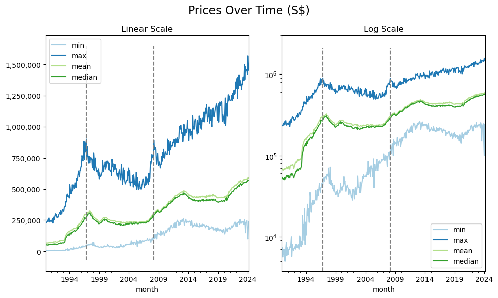
Looking at the graphs we see two points of interests around 1997 and 2008 where resale prices surged. Looking at the entire time period as a whole, resale prices have been steadying increasing over the past 30 years.
Before 2001, HDB flats were sold under the RFS scheme where flats were built ahead of time with with a surplus. In the few years leading up to the 1997 Asian Financial Crisis market conditions coupled with real estate speculation led to a surge in resale prices.
There was a surplus of ~31,000 units that took over 5 years to sell resulting in stagnating or even declining housing prices during this time. It was during this time that the BTO scheme was also introduced to combot the surplus problem, so flats were only built after enough units were purchased/registered.
Leading up to the 2008 Global Financial Crisis, housing prices surged once again reaching a local top before crashing slightly. However this time due to how heavily oversubscribed the BTO scheme was, demand for resale flats remained high and prices have been steadily increasing since.
tmp = df.groupby(['flat_type','month'])['resale_price'].agg(['min','max','mean','median']).reset_index()
for stat in ['min','max','mean','median']:
    fig, [ax1,ax2] = plt.subplots(2,1)
    sns.lineplot(data=tmp, x='month', y=stat, hue='flat_type', ax=ax1)
    sns.lineplot(data=tmp, x='month', y=stat, hue='flat_type', ax=ax2)
    ax2.set_yscale('log')

    ymin, ymax = f1.get_ylim()
    ax1.vlines(x=pd.to_datetime(['1996-11-01','2008-03-01']), ymin=ymin, ymax=ymax, colors=['tab:grey', 'tab:grey'], ls='--')
    ax1.set_ylim(top=tmp[stat].max(), bottom=tmp[stat].min())
    ymin, ymax = f2.get_ylim()
    ax2.vlines(x=pd.to_datetime(['1996-11-01','2008-03-01']), ymin=ymin, ymax=ymax, colors=['tab:grey', 'tab:grey'], ls='--')
    ax2.set_ylim(bottom=ymin)

    ax1.get_yaxis().set_major_formatter(
        mticker.FuncFormatter(lambda x, p: format(int(x), ',')))
    ax1.set_title('Linear Scale')
    ax2.set_title('Log Scale')
    fig.suptitle(f'{stat.capitalize()} Prices Over Time (S$)', fontsize=16)
    fig.set_size_inches(10,8)
    fig.tight_layout()
    fig.show()
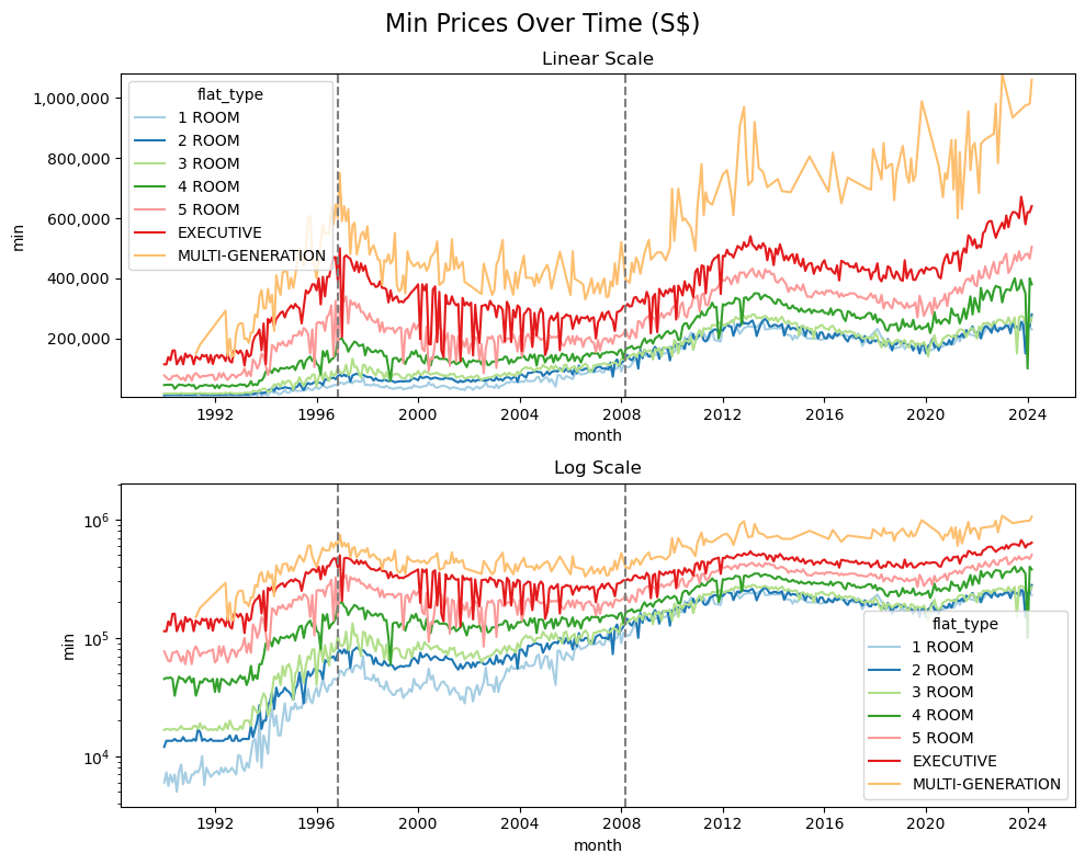
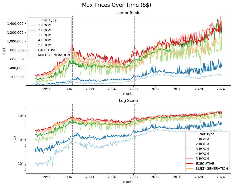
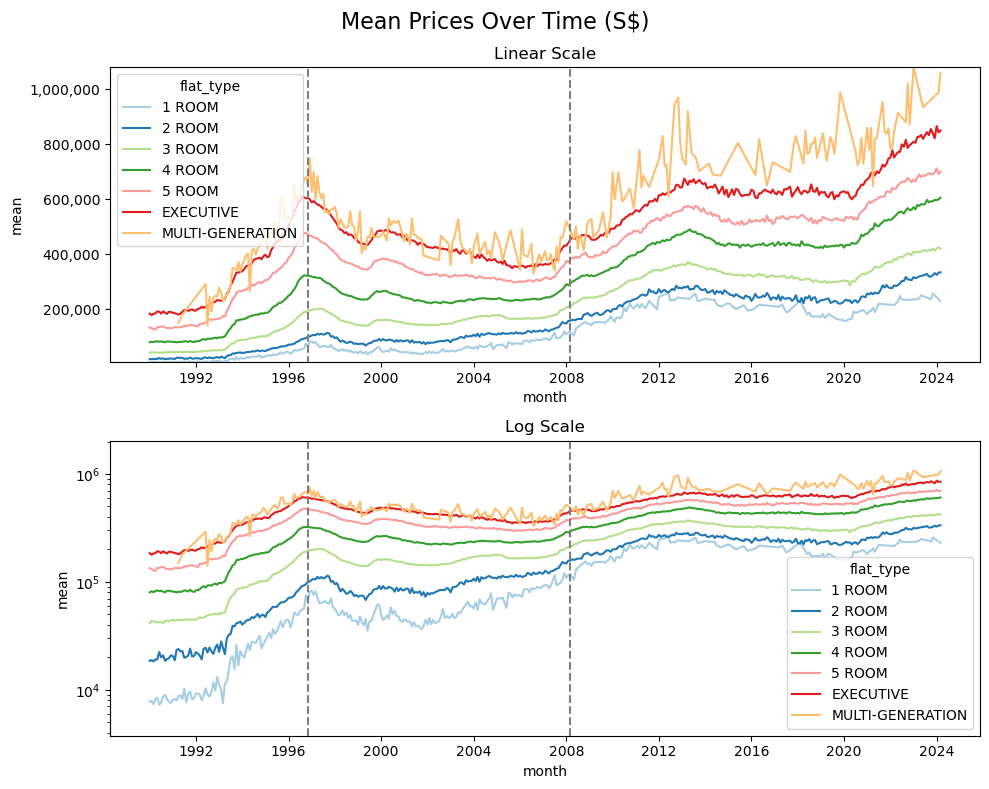
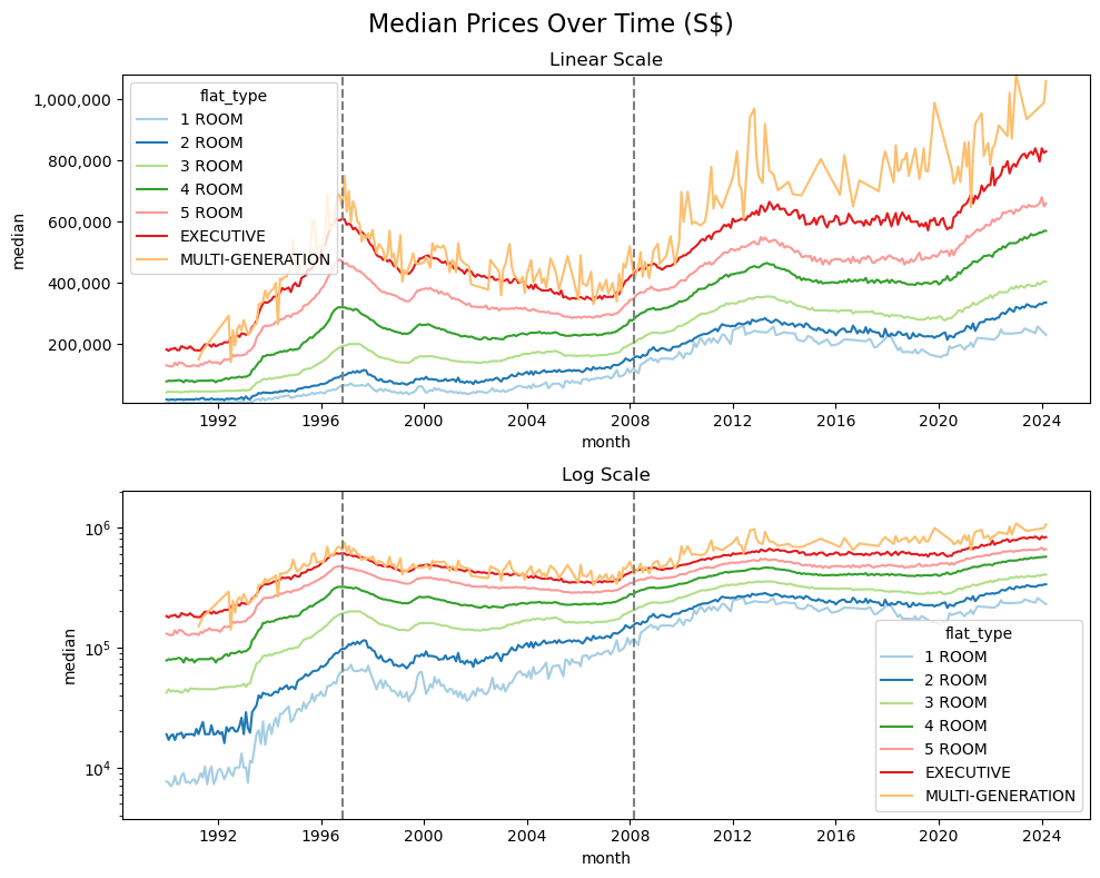
Price movements across the different flat types appear to be similar, with mean/median prices that are more representative of the flat type throughout the years. However when looking at max prices, 4room/5room/executive/multi-generation flats have been rapidly increasing since ~2008, with million dollar flats being sold since ~2014.
med = df.groupby(['flat_type','month'])['resale_price'].median().reset_index().set_index('month')

def plot_perc(ftype='3 ROOM'):
    tmp = med[med.flat_type==ftype]['resale_price'].resample('A').mean()
    tmp = tmp.reset_index()
    tmp['year'] = pd.PeriodIndex(tmp['month'], freq='A')
    tmp['year'] = pd.to_datetime(tmp['year'].astype(str)) + pd.offsets.YearEnd(0)
    tmp['change'] = tmp['resale_price'].pct_change() * 100
    tmp = tmp.fillna(0)
    #print(tmp)
    #print(tmp.dtypes)

    fig, ax = plt.subplots()
    a = sns.lineplot(data=tmp, x=pd.to_datetime(tmp['year']).dt.strftime('%Y'), y='change', ax=ax)
    x_dates = pd.to_datetime(tmp['year']).dt.strftime('%Y')
    #x_dates = ['' if i%4 else num for i,num in enumerate(x_dates)]
    ax.set_xticklabels(labels=x_dates, rotation=90, ha='right')
    ax.axhline(0, ls='--', color='tab:grey')

    fig.suptitle(f'Yearly Percentage Price Changes For {ftype.capitalize()} Flats (S$)', fontsize=16)
    fig.set_size_inches(12,6)
    fig.tight_layout()
    fig.show()
    return a

interact(plot_perc , ftype=ipywidgets.Dropdown(options=sorted(df.flat_type.unique())), value='3 ROOM', description='Flat Type: ')
interactive(children=(Dropdown(description='ftype', options=('1 ROOM', '2 ROOM', '3 ROOM', '4 ROOM', '5 ROOM',…


<function __main__.plot_perc(ftype='3 ROOM')>
The above function plots an interactive graph that allows user to switch between different flat types to observe the different price changes over the years. However it does not work on static webpages such as this one, hence a single graph showing the prices changes for 4 room flat type is shown instead.
plot_perc('4 ROOM')
<Axes: xlabel='year', ylabel='change'>
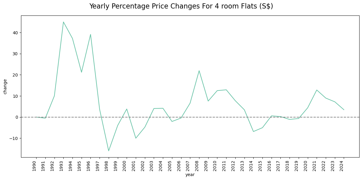
When looking at yearly mean percentage price changes, we see the similar patterns across all flat types. In the 1990s before 1997 there were large year on year increases (>60% for some years!). Between 2007 and 2013 there were also relatively large year on year increases across the flat types (>20% for some years).
In recent years the largest increases were between 2021-2023 presumably due to COVID restrictions putting a pause on BTO projects leading to increase demand for resale flats. Compared to the previous surges this appears to be a relatively smaller increase (>10%).
3.2 How does flat model, storey range, and size affect prices?
df
| month | town | flat_type | block | street_name | storey_range | floor_area_sqm | flat_model | lease_commence_date | remaining_lease | resale_price | lat | lng | yr | mth | |
|---|---|---|---|---|---|---|---|---|---|---|---|---|---|---|---|
| 0 | 1990-01-01 | ANG MO KIO | 1 ROOM | 309 | ANG MO KIO AVE 1 | mid_low | 31.0 | improved | 1977 | 86 | 9000.0 | 1.366059 | 103.836933 | 1990 | 1 |
| 1 | 1990-01-01 | ANG MO KIO | 1 ROOM | 309 | ANG MO KIO AVE 1 | low | 31.0 | improved | 1977 | 86 | 6000.0 | 1.366059 | 103.836933 | 1990 | 1 |
| 2 | 1990-01-01 | ANG MO KIO | 1 ROOM | 309 | ANG MO KIO AVE 1 | mid_low | 31.0 | improved | 1977 | 86 | 8000.0 | 1.366059 | 103.836933 | 1990 | 1 |
| 3 | 1990-01-01 | ANG MO KIO | 1 ROOM | 309 | ANG MO KIO AVE 1 | mid_low | 31.0 | improved | 1977 | 86 | 6000.0 | 1.366059 | 103.836933 | 1990 | 1 |
| 4 | 1990-01-01 | ANG MO KIO | 3 ROOM | 216 | ANG MO KIO AVE 1 | low | 73.0 | new generation | 1976 | 85 | 47200.0 | 1.366059 | 103.836933 | 1990 | 1 |
| ... | ... | ... | ... | ... | ... | ... | ... | ... | ... | ... | ... | ... | ... | ... | ... |
| 918190 | 2014-12-01 | YISHUN | 5 ROOM | 816 | YISHUN ST 81 | mid_low | 122.0 | improved | 1988 | 73 | 580000.0 | 1.414680 | 103.835299 | 2014 | 12 |
| 918191 | 2014-12-01 | YISHUN | EXECUTIVE | 325 | YISHUN CTRL | mid_low | 146.0 | maisonette | 1988 | 73 | 540000.0 | 1.414998 | 103.837006 | 2014 | 12 |
| 918192 | 2014-12-01 | YISHUN | EXECUTIVE | 618 | YISHUN RING RD | mid_low | 164.0 | apartment | 1992 | 77 | 738000.0 | 1.435217 | 103.836242 | 2014 | 12 |
| 918193 | 2014-12-01 | YISHUN | EXECUTIVE | 277 | YISHUN ST 22 | mid_low | 152.0 | maisonette | 1985 | 70 | 592000.0 | 1.437312 | 103.840977 | 2014 | 12 |
| 918194 | 2014-12-01 | YISHUN | EXECUTIVE | 277 | YISHUN ST 22 | low | 146.0 | maisonette | 1985 | 70 | 545000.0 | 1.437312 | 103.840977 | 2014 | 12 |
918195 rows × 15 columns
fig, [ax1,ax2] = plt.subplots(2,1, height_ratios=[1,2])
sns.countplot(data=df, x='flat_model', order = sorted(df.flat_model.unique()), ax=ax1)
ax1.set_yscale('log')
ax1.get_xaxis().set_visible(False)

sns.boxplot(data=df, x='flat_model', y='resale_price', order = sorted(df.flat_model.unique()), ax=ax2)
ax2.set_xticklabels(ax2.get_xticklabels(), rotation=45, ha='right')
ax2.axhline(df.resale_price.median(), ls='--', color='tab:grey')

ax2.get_yaxis().set_major_formatter(
    mticker.FuncFormatter(lambda x, p: format(int(x), ',')))
fig.set_size_inches(12,10)
fig.suptitle('Number of Flat Models in Dataset /\n Resale Prices of different Flat Models', fontsize=16)
fig.tight_layout()
fig.show()
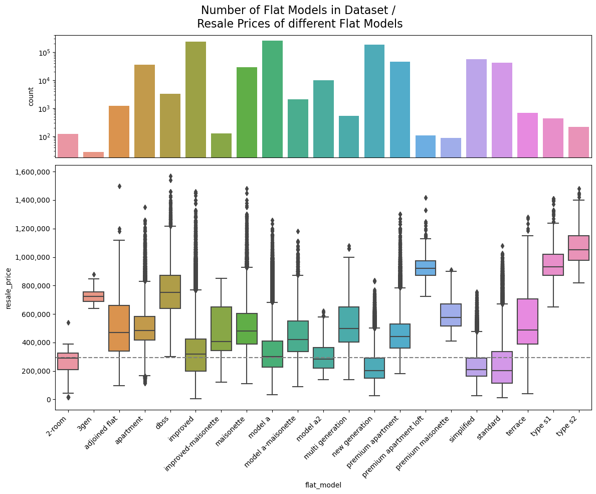
From the above graphs we see that apartment, improved, maisonette, model a, new generation, premium apartment, simplified, standard are the most popular/numerous resale flat model. Their price ranges are relatively close to the median prices of all resale flats.
In terms of prices we see that type s1, type s2, premium apartment loft are the most expensive. Coupled with their low supply, we can assume that these are premium flat models.
fig, [ax1,ax2] = plt.subplots(2,1, height_ratios=[1,2])
sns.countplot(data=df, x='storey_range', order=['low','mid_low','mid_high','high','very_high'], ax=ax1)
ax1.set_yscale('log')
ax1.get_xaxis().set_visible(False)

sns.violinplot(data=df, x='storey_range', y='resale_price', order=['low','mid_low','mid_high','high','very_high'], ax=ax2)
ax2.set_xticklabels(ax2.get_xticklabels(), rotation=45, ha='right')
ax2.axhline(df.resale_price.median(), ls='--', color='tab:grey')

ax2.get_yaxis().set_major_formatter(
    mticker.FuncFormatter(lambda x, p: format(int(x), ',')))
fig.set_size_inches(12,10)
fig.suptitle('Number of Storey Ranges in Dataset /\n Resale Prices of Different Storey Ranges', fontsize=16)
fig.tight_layout()
fig.show()
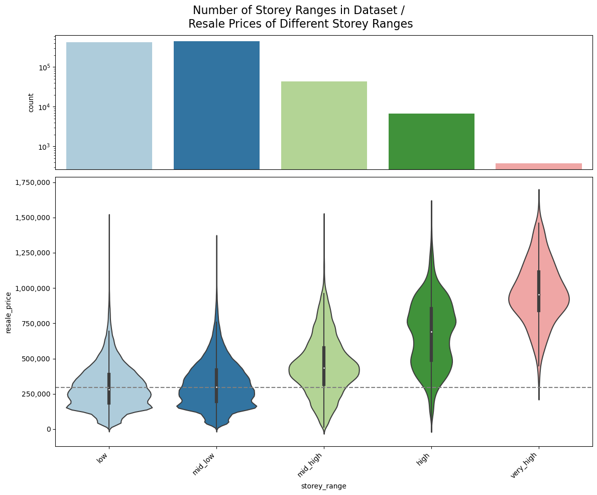
Looking at the graphs we see that low, mid_low flats makes up the majority of flats available, with price ranges close to the median price of all resale flats.
As the flats go higher we see the price trends high as well, up to a point where very_high flats (>40 storey) typically goes for almost triple the median price. This is ignoring the fact that these tall HDB buildings may be built in more desirable locations and are likely newer buildings, both of which will also contribute to a higher price.
def plot_scatter(x='floor_area_sqm', y='resale_price', year=2015):
    fig, ax = plt.subplots()
    a = sns.regplot(data=df[df.yr==year], x=x, y=y, ax=ax, line_kws={'color':'r'}, marker='.', order = 2)
    ax.set_xlim(left=max(0,(df.floor_area_sqm.min()-df.floor_area_sqm.std())), right=df.floor_area_sqm.max()+df.floor_area_sqm.std())
    ax.set_ylim(bottom=max(0,(df.resale_price.min()-df.resale_price.std())), top=df.resale_price.max()+df.resale_price.std())
    fig.set_size_inches(10,8)
    ax.get_yaxis().set_major_formatter(
        mticker.FuncFormatter(lambda x, p: format(int(x), ',')))
    fig.suptitle('Resale Price vs Floor Area(sqm) Across the Transaction Years')
    return a

interact(plot_scatter , year=ipywidgets.IntSlider(value=2015, min=df.yr.min(), max=df.yr.max(), step=1, description='Year'))
interactive(children=(Text(value='floor_area_sqm', description='x'), Text(value='resale_price', description='y…


<function __main__.plot_scatter(x='floor_area_sqm', y='resale_price', year=2015)>
The above function plots an interactive graph that allows user to switch between different years to observe the different resale_price/floor_area_sqm over the years. However it does not work on static webpages such as this one, hence a single graph for 2015 is shown instead.
plot_scatter()
<Axes: xlabel='floor_area_sqm', ylabel='resale_price'>
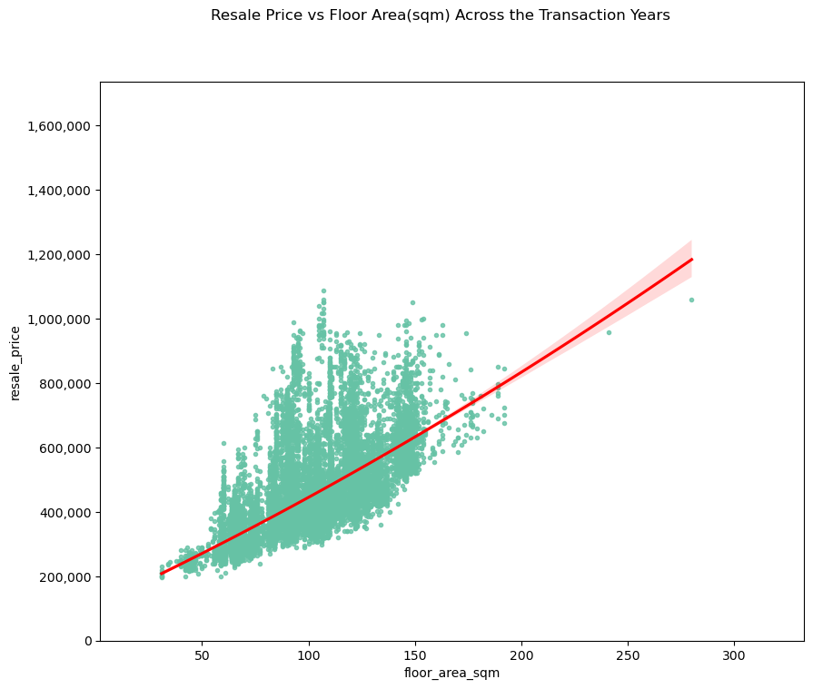
Looking at resale price vs floor area we see a positive correlation where bigger flat -> higher price across all transaction years.
3.3 How does location affect prices?
def plot_location(year=2015):
    fig, [ax1,ax2] = plt.subplots(2,1, height_ratios=[1,2])
    sns.countplot(data=df[df.yr==year], x='town', order=sorted(df.town.unique()), ax=ax1)
    #ax1.set_yscale('log')
    ax1.get_xaxis().set_visible(False)

    sns.boxplot(data=df[df.yr==year], x='town', y='resale_price', order=sorted(df.town.unique()), ax=ax2)
    ax2.set_xticklabels(ax2.get_xticklabels(), rotation=45, ha='right')
    ax2.axhline(df[df.yr==year].resale_price.median(), ls='--', color='tab:grey')

    ax2.get_yaxis().set_major_formatter(
        mticker.FuncFormatter(lambda x, p: format(int(x), ',')))
    fig.set_size_inches(12,10)
    fig.suptitle('Number of Flats in Town /\n Resale Prices of Flats in Different Towns', fontsize=16)
    fig.tight_layout()
    fig.show()

interact(plot_location , year=ipywidgets.IntSlider(value=2015, min=df.yr.min(), max=df.yr.max(), step=1, description='Year'))
interactive(children=(IntSlider(value=2015, description='Year', max=2024, min=1990), Output()), _dom_classes=(…


<function __main__.plot_location(year=2015)>
The above function plots an interactive graph that allows user to switch between different transaction years to observe the different geographical prices over the years. However it does not work on static webpages such as this one, hence a single graph showing the prices in 2015 is shown instead.
plot_location()
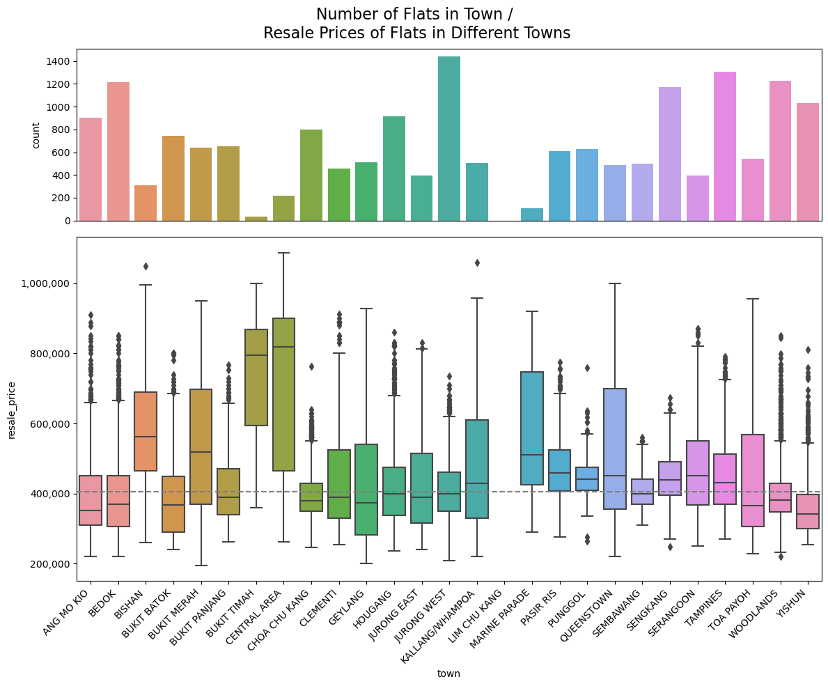
As expected, we see the most number of resale flats transacted in towns serving as larger population centres. The prices in these towns also range close to the median line.
Across the years the most expensive flats are typically found in towns where supply is relatively lower and/or the location is more desirable (central).
sns.set_palette("Set2")
fig, ax = plt.subplots(2,2, height_ratios=[1,2], width_ratios=[2,1], layout='compressed')
#sns.histplot(data=df, x='lng', kde=True, ax=ax[0,0])
sns.scatterplot(data=df, x='lng', y='resale_price', ax=ax[0,0])
sns.scatterplot(data=df, x='lng', y='lat', ax=ax[1,0])
#sns.histplot(data=df, y='lat', kde=True, ax=ax[1,1])
sns.scatterplot(data=df, x='resale_price', y='lat', ax=ax[1,1])

ax[0,0].get_xaxis().set_visible(False)
#ax[1,1].get_xaxis().set_visible(False)
ax[1,1].get_xaxis().set_major_formatter(
    mticker.FuncFormatter(lambda x, p: format(int(x), ',')))
#ax[0,0].get_yaxis().set_visible(False)
ax[0,0].get_yaxis().set_major_formatter(
    mticker.FuncFormatter(lambda x, p: format(int(x), ',')))
ax[1,1].get_yaxis().set_visible(False)
ax[0,1].set_visible(False)
ax[0,0].set_xlim(right=104.02)
ax[1,0].set_xlim(right=104.02)
ax[1,0].set_xticklabels(labels=np.linspace(103.65, 104.05, num=round((104.05-103.65)/0.05), endpoint=False))
fig.set_size_inches(10,8)
fig.tight_layout(pad=0.0)
fig.suptitle("Resale Prices Across Latitudes/Longitudes of Resale Flats", fontsize=16)
fig.show()
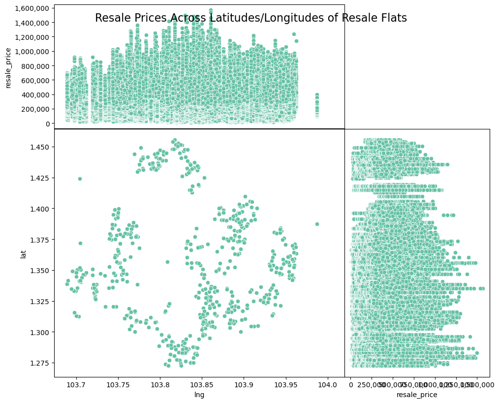
By combining 3 scatter plots to show the resale price per geographical coordinates, we observe that resale flats around the central / southern part of the island appear to fetch higher prices compared to other locations.
3.4 How does lease affect prices?
def plot_remaininglease(year=2015):
fig, ax = plt.subplots()
d = df[df.yr==year]
a = sns.regplot(data=d, x='remaining_lease', y='resale_price', ax=ax, line_kws={'color':'r'}, marker='.')
ax.set_xlim(left=max(0,(d.remaining_lease.min()-d.remaining_lease.std())), right=d.remaining_lease.max()+d.remaining_lease.std())
ax.set_ylim(bottom=max(0,(d.resale_price.min()-d.resale_price.std())), top=d.resale_price.max()+d.resale_price.std())
fig.set_size_inches(10,8)
ax.get_yaxis().set_major_formatter(
mticker.FuncFormatter(lambda x, p: format(int(x), ',')))
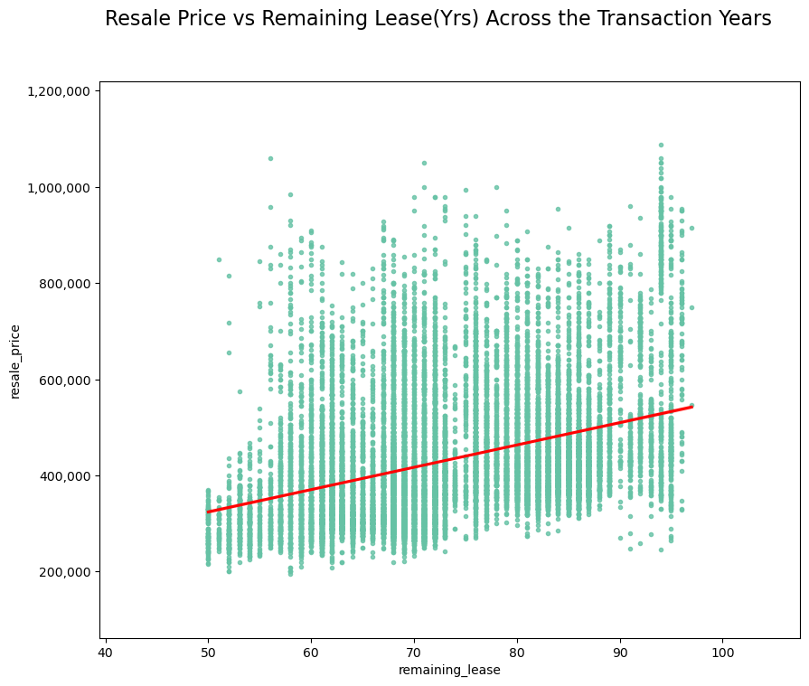
fig.suptitle('Resale Price vs Remaining Lease(Yrs) Across the Transaction Years', fontsize=16)
return a
interact(plot_remaininglease , year=ipywidgets.IntSlider(value=2015, min=df.yr.min(), max=df.yr.max(), step=1, description='Year'))
interactive(children=(IntSlider(value=2015, description='Year', max=2024, min=1990), Output()), _dom_classes=(…


<function __main__.plot_remaininglease(year=2015)>
The above code plots an interactive graph for users to select a transaction year to show the resale_price vs remaining_lease plot for. However as it requires an active kernel it cannot function on a static page hosted here on GitHub Pages. As an example I have shown a single plot for 2015 instead.
plot_remaininglease()
<Axes: xlabel='remaining_lease', ylabel='resale_price'>
def plot_commencelease(year=2015):
    fig, ax = plt.subplots()
    d = df[df.yr==year]
    a = sns.regplot(data=d, x='lease_commence_date', y='resale_price', ax=ax, line_kws={'color':'r'}, marker='.')
    ax.set_xlim(left=max(0,(d.lease_commence_date.min()-d.lease_commence_date.std())), right=d.lease_commence_date.max()+d.lease_commence_date.std())
    ax.set_ylim(bottom=max(0,(d.resale_price.min()-d.resale_price.std())), top=d.resale_price.max()+d.resale_price.std())
    fig.set_size_inches(10,8)
    ax.get_yaxis().set_major_formatter(
        mticker.FuncFormatter(lambda x, p: format(int(x), ',')))
    fig.suptitle('Resale Price vs Lease Commence Year Across the Transaction Years', fontsize=16)
    return a

interact(plot_commencelease , year=ipywidgets.IntSlider(value=2015, min=df.yr.min(), max=df.yr.max(), step=1, description='Year'))
interactive(children=(IntSlider(value=2015, description='Year', max=2024, min=1990), Output()), _dom_classes=(…


<function __main__.plot_commencelease(year=2015)>
Similarly, the above code plots an interactive graph for resale_price vs lease_commence_date that does not function on a static webpage. As an example I have plotted the graph for 2015.
plot_commencelease()
<Axes: xlabel='lease_commence_date', ylabel='resale_price'>
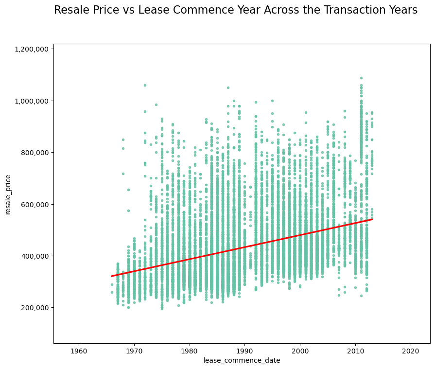
Looking at resale prices vs remaining lease / lease commencement year across all the transaction years, we observe that prices are correlated with newer flats or flats with a longer remaining lease. Newer flats are sold for anywhere between 50% to 300% more than old flats depending on the year of transaction, with the disparity shrinking in recent years.
3.5 Are flats getting smaller?
def plot_area(ftype='3 ROOM'):
fig, ax = plt.subplots(2,1, height_ratios=[1,2])
d = df[df.flat_type==ftype]
c = df[df.flat_type==ftype][['lease_commence_date','flat_type']]
l=max(0,(d.lease_commence_date.min()-d.lease_commence_date.std()))
r=d.lease_commence_date.max()+d.lease_commence_date.std()
b = sns.histplot(data=c, x=c.lease_commence_date, ax=ax[0], bins=int(r-l))
a = sns.regplot(data=d, x='lease_commence_date', y='floor_area_sqm', ax=ax[1], line_kws={'color':'r'}, marker='.', order=3)
ax[0].get_xaxis().set_visible(False)
ax[0].set_xlim(left=l, right=r)
ax[1].set_xlim(left=l, right=r)
ax[1].set_ylim(bottom=max(0,(d.floor_area_sqm.min()-d.floor_area_sqm.std())), top=d.floor_area_sqm.max()+d.floor_area_sqm.std())
fig.set_size_inches(10,8)
ax[1].get_yaxis().set_major_formatter(
mticker.FuncFormatter(lambda x, p: format(int(x), ',')))
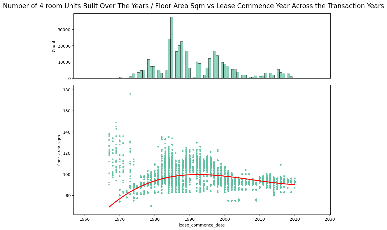
fig.suptitle(f'Number of {ftype.capitalize()} Units Built Over The Years / Floor Area Sqm vs Lease Commence Year Across the Transaction Years', fontsize=16)
fig.tight_layout()
return a
interact(plot_area , ftype=ipywidgets.Dropdown(options=sorted(df.flat_type.unique())), value='3 ROOM', description='Flat Type: ')
interactive(children=(Dropdown(description='ftype', options=('1 ROOM', '2 ROOM', '3 ROOM', '4 ROOM', '5 ROOM',…


<function __main__.plot_area(ftype='3 ROOM')>
The above function plots an interactive graph that allows user to switch between flat types to observe the different floor_area_sqm/lease_commence_date over the years. However it does not work on static webpages such as this one, hence a single graph for 4 room flat type is shown instead.
plot_area('4 ROOM')
<Axes: xlabel='lease_commence_date', ylabel='floor_area_sqm'>
df.flat_type.value_counts()
flat_type
4 ROOM              348948
3 ROOM              292893
5 ROOM              193761
EXECUTIVE            69215
2 ROOM               11595
1 ROOM                1242
MULTI-GENERATION       541
Name: count, dtype: int64
3/4/5/Executive room flat types makes up the vast majority (>98%) of resale flat transactions, with the other flat types the number of units being built and transacted over the past 60 years may be too few to generalize conclusions.
Looking at the floor area of the different flat types over the years, in general flats above 4 room built between 1980~2000 were around 10% larger than flats built in the 2020s, and bulk of the resale units were also built in the same period.
plot_area('3 ROOM')
<Axes: xlabel='lease_commence_date', ylabel='floor_area_sqm'>
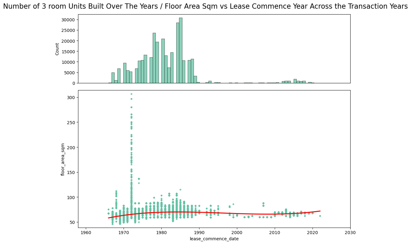
df[(df.flat_type=='3 ROOM')&(df.floor_area_sqm > 110)]['flat_model'].value_counts()
flat_model
terrace     224
improved     16
model a       1
Name: count, dtype: int64
When looking at 3 room flat types almost all the units were built between 1970~1990 with a small number of units being built in the 2010s. The newer units for this flat type does not appear to be any smaller/larger than the old units.
There are a small number of 3 room units built in the 1970s that goes up to 4x the size of an average 3 room unit. These are special HDB landed properties that only number in the hundreds and do not affect the analysis of flat sizes.